Selfish Equity & Capital Market Equilibrium

Social Finance -- Online Appendix and Notebook 4

This notebook implements the Selfish Equity extension of the social finance model described in Section 6 and Appendix B of the paper main.tex.

Theoretical Background¶

In our baseline model (explored in 2-socfin_m.ipynb), we assumed a highly competitive or altruistic market where the opportunity cost of MFI monitoring equity capital $\beta$ was exactly equal to the cost of uninformed debt capital $\gamma$ (i.e. $\beta = \gamma = 1.0$ ).

However, in most real-world contexts, informed monitoring capital is highly scarce. Specialized managers, loan officers, and screeners represent scarce resources. Under a commercial or profit-driven intermediation regime, monitoring equity investors demand an expected rate of return on their equity capital in excess of the cost of debt:

\beta > \gamma

(1)

This ROE hurdle rate $\beta$ introduces two critical economic frictions:

“Wasteful Over-Monitoring”: To deliver a higher expected return $\beta$ to the monitor while maintaining borrower incentives, the contract must adjust. For any given level of pledgeable assets $A$ , borrowers are subjected to more intensive active monitoring $m$ than they would choose under a competitive or social lender.
“Leverage Rationing”: To keep the monitor’s incentives credible under a high return rate $\beta$ , the monitor must retain a deeper equity stake $I^m$ in each loan. Furthermore, the loan fixed operational cost $f$ must always be financed out of MFI equity capital (at opportunity cost $\beta$ ). Thus, the total MFI equity per loan is:
$I^m_{\text{total}}(A, \beta) = I^m(A, \beta) + f$
(2)
where $I^m(A, \beta) = \frac{1}{\beta} \frac{q \cdot m(A)}{p - q}$ . The leverage ratio (debt-to-equity) is therefore:
$\text{D/E} = \frac{I - I^m}{I^m + f}$
(3)
As the required ROE $\beta$ rises, the MFI is forced to hold more skin in the game, restricting its ability to leverage outside commercial funds and limiting its borrower outreach $N$ .

Natural Leverage Bounds¶

Since $I^m \ge 0$ , this formulation naturally bounds the maximum leverage ratio at:

\text{Max D/E} = \frac{I}{f} = \frac{100}{20} = 5.0

(4)

This bounds leverage using only the physical parameters of the loan ( $I$ and $f$ ), without needing an ad-hoc regulatory Capital Adequacy Ratio (CAR) constraint.

Economy-Wide Equilibrium¶

By “closing the model”, we solve for the economy-wide equilibrium return on equity $\beta^*$ that clears the market for a fixed total supply of informed capital $K_{total}$ . As $\beta$ rises, credit access falls and the demand for capital shrinks, yielding a unique market-clearing interest rate for social and commercial finance.

%matplotlib inline
import sys
import os
import numpy as np
import matplotlib.pyplot as plt
from ipywidgets import interact, FloatSlider
from scipy.optimize import root_scalar

# Path configuration to find local packages
sys.path.append(os.path.abspath('..'))

# Autoreload settings useful while editing socialfinance.py
%load_ext autoreload
%autoreload 2

# Matplotlib styling
plt.rcParams['figure.figsize'] = (7.5, 5.5)
plt.rcParams['axes.grid'] = True
plt.rcParams['grid.linestyle'] = ':'
plt.rcParams['grid.alpha'] = 0.6

# Import the core Bank class
from socialfinance.socialfinance import Bank

Let’s visualize the impact of commercial ROE hurdles. We will compare a Baseline MFI accepting a return on equity exactly equal to the cost of debt ( $\beta = \gamma = 1.0$ ) with a series of Commercial MFIs requiring ROE hurdle rates ranging from $10\%$ to $50\%$ (i.e. $\beta = 1.1, 1.2, 1.3, 1.4, 1.5$ ).

The minimum collateral requirement for a leveraged MFI under selfish equity is:

AM(m) = \frac{p}{p-q} B(m) - (p X - \gamma I - \beta f) + m + \frac{\beta - \gamma}{\beta} \frac{q m}{p-q}

(5)

And the minimum collateral for an equity-only MFI is:

AMe(m) = \frac{p}{p-q} B(m) - (p X - \beta(I + f)) + m

(6)

Let’s initialize a range of pledgeable assets $A$ and create our MFI zones.

--- Model Parameters ---
Amax = 140, B0 = 30, F = 0, I = 100, K = 10000, X = 200
alpha = 0.5, beta = 1.0, f = 20, gamma = 1.0, p = 0.97, q = 0.82

The Contract Space Envelope & Over-monitoring¶

The solid envelope represents the feasible contract frontier (the minimum collateral pledge required for each level of monitoring $m$ ).

Notice that as the required ROE $\beta$ shifts from the baseline 1.0 (blue) to the commercial steps from 1.1 to 1.5 (red gradient):

The minimum collateral requirement curve $A(m)$ shifts upward.
The crossover point $m_{cross}$ where the leveraged MFI and equity-only MFI cross shifts to the right.
This means that for any given asset level, commercial borrowers are subjected to progressively higher monitoring intensity $m$ and therefore higher interest rates to cover the monitor’s high ROE.

fig, ax = plt.subplots(figsize=(8.5, 6.5))
mm = np.linspace(0, 80, 500)

# Plot the A_e(m) and A(m) baseline (beta=gamma=1.0)
ax.plot(mm, mfi_baseline.AMe(mm), linewidth=3.2, color='blue', label=r'Baseline MFI ($\beta = 1.0$)')

# Use a colormap to plot beta steps from 1.1 to 1.5
import matplotlib.cm as cm
betas = [1.1, 1.2, 1.3, 1.4, 1.5]
colors = cm.Reds(np.linspace(0.4, 1.0, len(betas)))

for b, color in zip(betas, colors):
    mfi_temp = Bank(A, beta=b)
    mmax_temp = mfi_temp.mmax()
    if mmax_temp > 0:
        mm_env = np.linspace(0, mmax_temp, 500)
        ax.plot(mm_env, mfi_temp.Abest(mm_env), linewidth=1.8, color=color, linestyle='--',
                label=rf'Commercial $\beta = {b:.1f}$ (ROE = {(b-1.0)*100:.0f}%)')

ax.set_title("Minimum Collateral Requirements: Over-Monitoring under Hurdle ROE", fontsize=12, weight='bold')
ax.set_xlabel("Monitoring intensity $m$", fontsize=10)
ax.set_ylabel("Pledgeable assets $A(m)$", fontsize=10)
ax.set_xlim(0, 80)
ax.set_ylim(0, 160)
ax.legend(fontsize=9, loc='upper right')
plt.tight_layout()
os.makedirs('figs', exist_ok=True)
plt.savefig('figs/fig-crossover-compare.png', dpi=300)
plt.show()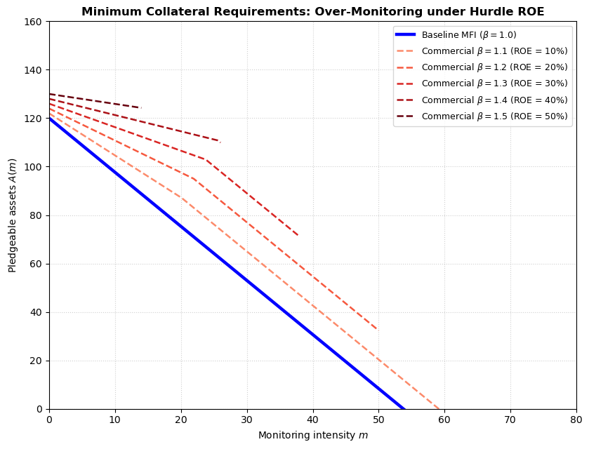

Leverage Rationing & Debt-to-Equity Compression¶

As the MFI’s hurdle ROE $\beta$ rises, outside uninformed investors demand that the MFI invest more of its own capital $I^m$ per loan to align incentives. Since operational cost $f$ is equity-financed, the leverage ratio collapses.

The plot below maps the debt-to-equity ratio across different pledgeable asset levels. Note how the commercial leverage curves (red gradient) sit significantly below the baseline, and are naturally capped at $I/f = 5.0$ , showing how commercial profit-maximizing hurdles restrict leverage and limit the scale of financial inclusion.

fig, ax = plt.subplots(figsize=(8.5, 6.0))

# Baseline (beta = 1.0) - leverage is capped at I/f under equity-funded operational cost f
# Plot the leverage curves for beta steps from 1.1 to 1.5
import matplotlib.cm as cm
betas = [1.1, 1.2, 1.3, 1.4, 1.5]
colors = cm.Reds(np.linspace(0.4, 1.0, len(betas)))

for b, color in zip(betas, colors):
    mfi_temp = Bank(A, beta=b)
    amin_temp = mfi_temp.Amin()
    A_temp = np.linspace(amin_temp, mfi_temp.AM(0), 100)[:-1]
    Im_temp = np.array([mfi_temp.Im(m) for m in mfi_temp.minmon(A_temp)])
    de_temp = np.divide(mfi_temp.I - Im_temp, Im_temp + mfi_temp.f, out=np.zeros_like(Im_temp), where=(Im_temp + mfi_temp.f)>0)
    
    ax.plot(A_temp, de_temp, label=rf'Commercial $\beta = {b:.1f}$ (ROE = {(b-1.0)*100:.0f}%)', color=color, linewidth=2)
    ax.axvline(x=mfi_temp.Across(), linestyle=':', color=color, alpha=0.6)

# Draw the natural leverage limit line
max_de = mfi_baseline.I / mfi_baseline.f
ax.axhline(y=max_de, color='red', linestyle='--', linewidth=2, alpha=0.7, label=f'Max Leverage ({max_de:.1f})')

ax.set_title(r"Debt-to-Equity Ratio $\frac{I - I^m}{I^m + f}$ under Scarce Equity and Operational Cost $f$", fontsize=12, weight='bold')
ax.set_xlabel("A -- pledgeable assets", fontsize=10)
ax.set_ylabel("Leverage Ratio", fontsize=10)
ax.set_xlim(20, 140)
ax.set_ylim(0, max_de * 1.25)  # dynamically sets y-limit to exactly 1.25 times the cap (6.25)
ax.legend(fontsize=9, loc='upper right')
plt.tight_layout()
plt.savefig('figs/fig-leverage-rationing.png', dpi=300)
plt.show()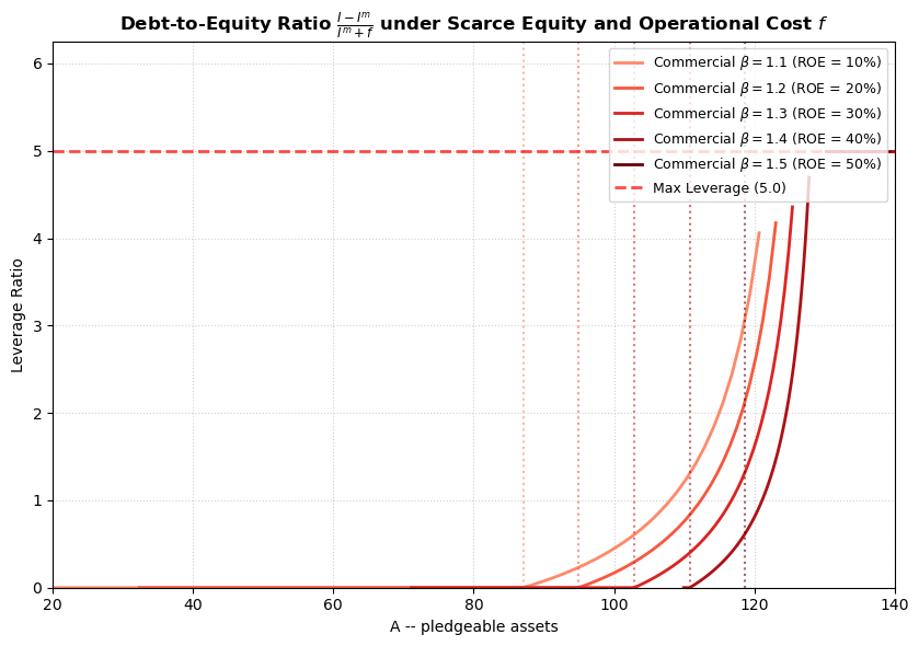

2. Closing the Model: Solving for Equilibrium ROE $\beta^*$ ¶

Now we will implement the general equilibrium module that clears the capital market for MFI monitoring equity.

Market-Clearing Mechanics¶

Let there be a continuum of segregated neighborhoods indexed by average wealth $A_j \in [0, 150]$ . Each neighborhood has $N_{potential}$ potential borrowers.

The MFI equity capital used in neighborhood $A_j$ for a given ROE $\beta$ is:

K_j(A_j, \beta) = N_{potential} \cdot (I^m(A_j, \beta) + f)

(7)

The total economy-wide MFI equity capital demanded is:

K_{demand}(\beta) = \sum_{j} N_{potential} \cdot (I^m(A_j, \beta) + f)

(8)

We define a vectorized function to compute $K_{demand}(\beta)$ and solve for the equilibrium $\beta^*$ that satisfies $K_{demand}(\beta^*) = K_{total}$ .

# Neighborhoods and borrowers setup
beta_vals = np.linspace(1.0, 2.0, 100)
A_grid = np.linspace(0, 150, 1000)
N_potential = 20.0  # potential borrowers per neighborhood
K_total = 500000.0  # Total economy-wide supply of intermediary equity capital

# Solve the model using refactored Bank class methods
beta_star = Bank.solve_equilibrium(A_grid, K_total, N_potential, bracket=[1.0, 2.5])

print(f"Market-Clearing Equilibrium ROE (beta*) = {beta_star:.5f}")

Market-Clearing Equilibrium ROE (beta*) = 1.34073

kd_vals = [Bank(A_grid, beta=b).capital_demand_grid(A_grid, N_potential) for b in beta_vals]

fig, ax = plt.subplots(figsize=(8, 5.5))
ax.plot(kd_vals, beta_vals, label=r"Capital Demand", color='purple', linewidth=2.5)
ax.axvline(x=K_total, color='green', linestyle='--', linewidth=2, label=r"Capital Supply $K_{total}$")

ax.plot(K_total, beta_star, 'ro', markersize=9, label=rf"Equilibrium ($\beta^* = {beta_star:.3f}$)")

ax.set_title("Equilibrium Return on Intermediary Capital", fontsize=12, weight='bold')
ax.set_xlabel("Total MFI Capital demanded / supplied", fontsize=10)
ax.set_ylabel(r"Return on Intermediary Equity $\beta$", fontsize=10)
ax.legend(fontsize=10)
plt.tight_layout()
plt.savefig('figs/fig-equilibrium-clearing.png', dpi=300)
plt.show()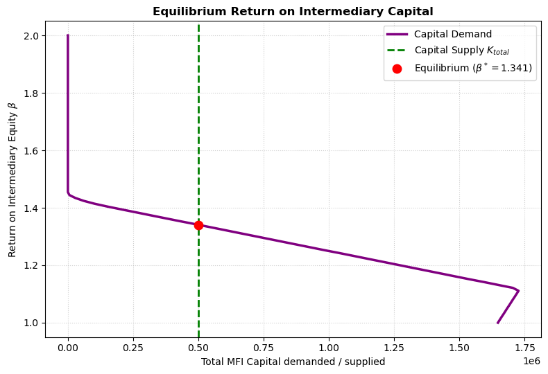

3. The Equilibrium Credit Landscape¶

Using our equilibrium ROE $\beta^*$ , let’s analyze the resulting credit landscape. We will plot the lending outreach (number of borrowers reached $N(A)$ ) and the borrower net returns (welfare surplus) across the wealth distribution.

# Initialize the bank under equilibrium beta*
eq_bank = Bank(A, beta=beta_star)
eq_bank.K = 10000.0  # MFI startup capital parameter

# Calculate borrower outreach N(A) and net returns
nr = eq_bank.nreach(A)
br = eq_bank.breturn(A)

fig, (ax1, ax2) = plt.subplots(2, 1, figsize=(8.5, 9.5))

# Plot 1: Outreach
ax1.plot(A, nr, color='teal', linewidth=3, label='Equilibrium Outreach $N(A)$')
ax1.axvline(x=eq_bank.Amin(), linestyle=':', color='grey', label='Excluded threshold')
ax1.axvline(x=eq_bank.Across(), linestyle=':', color='blue', label='Leverage threshold')
ax1.axvline(x=eq_bank.AM(0), linestyle=':', color='green', label='Direct banking threshold')
ax1.set_title("Equilibrium MFI Outreach by Borrower Asset Level", fontsize=11, weight='bold')
ax1.set_xlabel("Borrower pledgeable assets $A$", fontsize=9)
ax1.set_ylabel("Number of loans funded ($N$)", fontsize=9)
ax1.set_xlim(0, 140)
ax1.set_ylim(0, 350)
ax1.legend(fontsize=9)

# Plot 2: Borrower returns
ax2.plot(A, br, color='orange', linewidth=3, label='Borrower net return')
ax2.axvline(x=eq_bank.Amin(), linestyle=':', color='grey')
ax2.axvline(x=eq_bank.Across(), linestyle=':', color='blue')
ax2.axvline(x=eq_bank.AM(0), linestyle=':', color='green')
ax2.set_title("Equilibrium Borrower Returns by Asset Level", fontsize=11, weight='bold')
ax2.set_xlabel("Borrower pledgeable assets $A$", fontsize=9)
ax2.set_ylabel("Expected Net Surplus", fontsize=9)
ax2.set_xlim(0, 140)
ax2.set_ylim(0, 120)
ax2.legend(fontsize=9)

plt.tight_layout()
plt.savefig('figs/fig-equilibrium-landscape.png', dpi=300)
plt.show()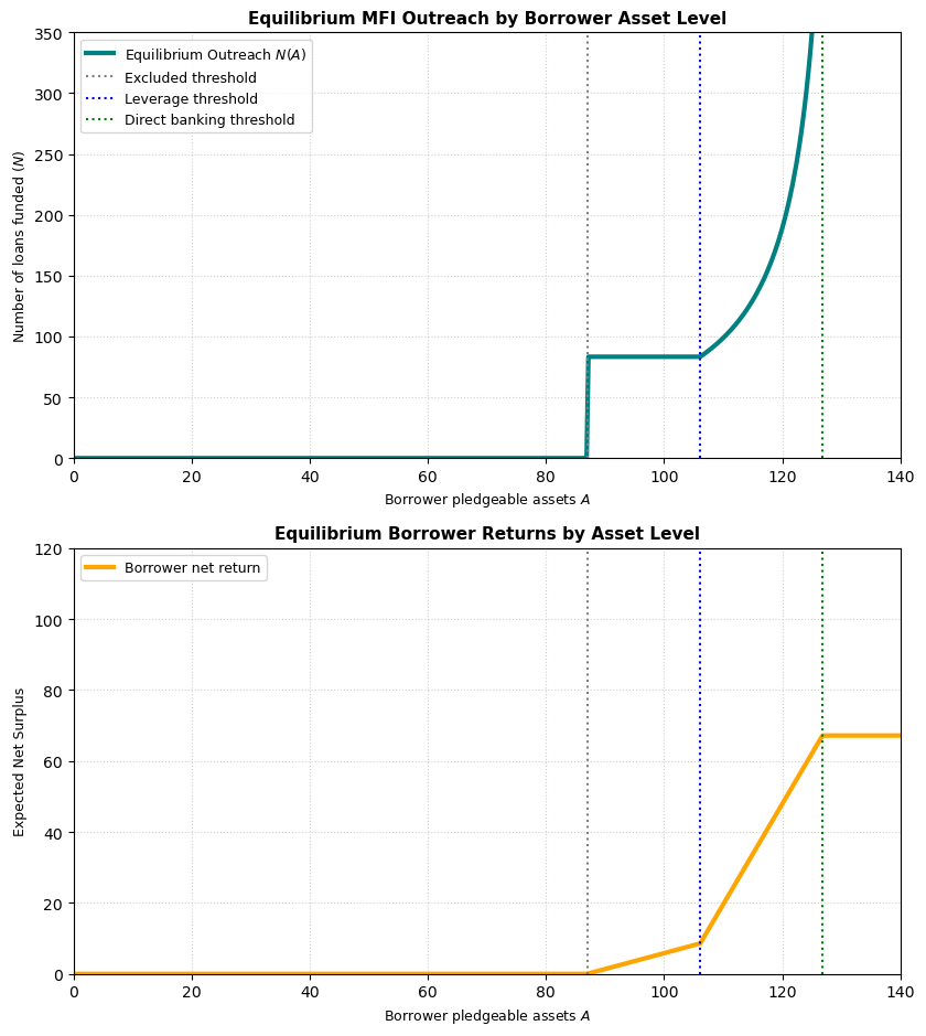

4. Interactive Capital Market & Policy Dashboard¶

Use the interactive dashboard below to explore in real-time how the capital market clears! You can vary the total intermediary capital supply ( $K_{total}$ ), the cost of uninformed debt ( $\gamma$ ), the monitoring efficiency ( $\alpha$ ), and the MFI fixed operational cost ( $f$ ).

The dashboard dynamically resolves the market-clearing equilibrium rate of return $\beta^*$ and updates the contract space plots instantly.

def interactive_equilibrium(K_total_val=400000.0, gamma_val=1.0, alpha_val=0.5, f_val=20.0):
    # Close previous plots to avoid memory leakage
    plt.close('all')
    from IPython.display import clear_output
    clear_output(wait=True)
    
    # Solve for equilibrium under new parameters using refactored Bank class methods
    try:
        b_star = Bank.solve_equilibrium(
            A_grid, K_total_val, N_potential=N_potential, bracket=[1.0, 3.0],
            gamma=gamma_val, alpha=alpha_val, f=f_val
        )
    except ValueError:
        print("Market collapsed: Intermediary capital demand cannot match supply in this range.")
        return
        
    # Display solved value
    from IPython.display import display, Markdown
    display(Markdown(f"### **Solved Equilibrium Rate:** $\\beta^* = {b_star:.4f}$ (ROE = {(b_star-1.0)*100:.2f}%)"))
    
    # Draw the dynamic plots side-by-side (3-column layout)
    fig, (ax1, ax2, ax3) = plt.subplots(1, 3, figsize=(18, 5.5))
    
    # Left Plot: Capital Market Clearing
    b_test_range = np.linspace(1.0, 2.5, 50)
    kd_test_vals = []
    for b in b_test_range:
        tb = Bank(A_grid, beta=b, gamma=gamma_val, alpha=alpha_val, f=f_val)
        kd_test_vals.append(tb.capital_demand_grid(A_grid, N_potential))
        
    ax1.plot(kd_test_vals, b_test_range, color='purple', linewidth=2.5, label='Capital Demand')
    ax1.axvline(x=K_total_val, color='green', linestyle='--', linewidth=2, label='Capital Supply')
    ax1.plot(K_total_val, b_star, 'ro', markersize=9, label=rf'Equilibrium $\beta^*={b_star:.2f}$')
    ax1.set_title("Intermediary Capital Market Clearing", fontsize=12, weight='bold')
    ax1.set_xlabel("Total MFI Capital demanded / supplied", fontsize=10)
    ax1.set_ylabel(r"Return on Equity $\beta$", fontsize=10)
    ax1.legend()
    
    # Center Plot: Resulting Contract Envelope
    eq_mfi = Bank(A, beta=b_star, gamma=gamma_val, alpha=alpha_val, f=f_val)
    
    mm_range = np.linspace(0, 100, 500)
    ax2.plot(mm_range, eq_mfi.AMe(mm_range), linestyle=':', color='green', alpha=0.5, label='Equity-only MFI')
    ax2.plot(mm_range, eq_mfi.AM(mm_range), linestyle='--', color='purple', alpha=0.5, label='Leveraged MFI')
    
    mmax_val = eq_mfi.mmax()
    if mmax_val > 0:
        mm_env = np.linspace(0, mmax_val, 200)
        ax2.plot(mm_env, eq_mfi.Abest(mm_env), linewidth=3, color='blue', label='Feasible Frontier')
        ax2.axvline(x=mmax_val, linestyle='--', color='red', alpha=0.6, label='Max monitoring limit')
        
    ax2.set_title(r"Resulting Equilibrium Contract Space $A(m)$", fontsize=12, weight='bold')
    ax2.set_xlabel("Monitoring intensity $m$", fontsize=10)
    ax2.set_ylabel("Pledgeable assets $A(m)$", fontsize=10)
    ax2.set_xlim(0, 80)
    ax2.set_ylim(0, 160)
    ax2.legend()
    
    # Right Plot: Resulting Debt-to-Equity Ratio
    amin_eq = eq_mfi.Amin()
    A_temp = np.linspace(amin_eq, eq_mfi.AM(0), 100)[:-1]
    Im_temp = np.array([eq_mfi.Im(m) for m in eq_mfi.minmon(A_temp)])
    de_temp = np.divide(eq_mfi.I - Im_temp, Im_temp + eq_mfi.f, out=np.zeros_like(Im_temp), where=(Im_temp + eq_mfi.f)>0)
    
    ax3.plot(A_temp, de_temp, color='blue', linewidth=2.5, label='D/E Ratio')
    ax3.axvline(x=eq_mfi.Amin(), color='grey', linestyle=':', alpha=0.7, label=r'$A_{min}$')
    ax3.axvline(x=eq_mfi.Across(), color='blue', linestyle=':', alpha=0.7, label=r'$A_{cross}$')
    ax3.axvline(x=eq_mfi.AM(0), color='green', linestyle=':', alpha=0.7, label=r'$A(0)$')
    
    max_de = eq_mfi.I / eq_mfi.f
    ax3.axhline(y=max_de, color='red', linestyle='--', linewidth=2, alpha=0.7, label=f'Max Leverage ({max_de:.1f})')
    y_max = max_de * 1.25
        
    ax3.set_title("Resulting Debt-to-Equity Ratio", fontsize=12, weight='bold')
    ax3.set_xlabel("A -- pledgeable assets", fontsize=10)
    ax3.set_ylabel("Leverage Ratio", fontsize=10)
    ax3.set_xlim(amin_eq - 15, 140)
    ax3.set_ylim(0, y_max)
    ax3.legend(fontsize=9, loc='upper right')
    
    plt.tight_layout()
    plt.show()

# Interactive control sliders
interact(interactive_equilibrium,
         K_total_val=FloatSlider(min=200000.0, max=600000.0, step=25000.0, value=400000.0, description='Capital Supply'),
         gamma_val=FloatSlider(min=1.0, max=1.2, step=0.02, value=1.0, description='Debt Cost gamma'),
         alpha_val=FloatSlider(min=0.3, max=0.7, step=0.05, value=0.5, description='Monitoring alpha'),
         f_val=FloatSlider(min=0.0, max=30.0, step=5.0, value=20.0, description='Fixed Cost f'));