Social Finance -- Online Appendix and Notebook 6
This notebook implements the general equilibrium model of a social and commercial banking market clearing when project returns follow a Pareto distribution:
Unlike the Uniform distribution in 5-endogenous-NK.ipynb, the Pareto distribution is highly right-skewed with most project returns concentrated near the minimum value and a long, thin tail of highly productive projects. This creates a very different spatial capital allocation profile, where commercial MFIs strongly concentrate their scarce capital in wealthier areas.
Source
import sys
import os
import numpy as np
import matplotlib
# matplotlib.use('Agg')  # non-interactive backend for batch execution
import matplotlib.pyplot as plt
import matplotlib.cm as cm
from scipy.optimize import root_scalar, brentq
from scipy.integrate import quad

# Path configuration to find local packages
sys.path.append(os.path.abspath('..'))

# Matplotlib styling
plt.rcParams['figure.figsize'] = (8.5, 6.0)
plt.rcParams['axes.grid'] = True
plt.rcParams['grid.linestyle'] = ':'
plt.rcParams['grid.alpha'] = 0.6
plt.rcParams['font.size'] = 11

# Import the core Bank class
from socialfinance.socialfinance import Bank, BankHetX

os.makedirs('figs', exist_ok=True)
print('Imports complete.')
Imports complete.
1. Analytical Foundations
The Pareto Model
We assume that within each neighborhood (characterized by pledgeable assets ), there is a finite population of potential borrowers. Each borrower has a project with success return drawn i.i.d. from a common Pareto distribution:
The cumulative distribution function is:
Modified Contract Equations
The minimum collateral requirement under leveraged intermediation remains:
The MFI serves borrowers with , where .
Outreach & Capital Demand under Pareto
Because follows a Pareto distribution, the fraction of the population served in neighborhood is:
The aggregate MFI capital demand in neighborhood is computed by integrating the required skin-in-the-game equity over the Pareto density from to :
We have derived the closed-form analytical integral for this demand:
where and .
2. Validation: Recovering the Baseline
Before exploring the new model, let’s verify that BankHetX recovers the baseline when degenerates to a point mass at . We also verify the analytical formula against numerical root-finding.
Source
import numpy as np
from socialfinance.socialfinance import BankHetX

A_test = np.array([30.0, 60.0, 90.0, 120.0])
beta_test = 1.2

# BankHetX under Pareto with X_m = 160, alpha_pareto = 3.0
bank_het = BankHetX(A_test, beta=beta_test, dist_type='pareto', X_m=160, alpha_pareto=3.0)

print("=== Validation: Pareto Cutoffs ===")
for a in A_test:
    xs_star = bank_het.X_star(a)
    xs_nm = bank_het.X_no_monitoring(a)
    frac = bank_het.frac_served(a)
    print(f"A_j = {a:.1f}: X_star = {xs_star:.2f}, X_nm = {xs_nm:.2f}, Fraction served = {frac:.4f}")
=== Validation: Pareto Cutoffs ===
A_j = 30.0: X_star = 223.64, X_nm = 292.78, Fraction served = 0.3662
A_j = 60.0: X_star = 205.36, X_nm = 261.86, Fraction served = 0.4729
A_j = 90.0: X_star = 187.08, X_nm = 230.93, Fraction served = 0.6255
A_j = 120.0: X_star = 168.80, X_nm = 200.00, Fraction served = 0.8516
3. The Credit Demand Curve Within a Neighborhood
For a single neighborhood , we can now visualize the intensive margin: how the MFI’s lending expands as it dips deeper into the distribution.
For each served borrower, we plot:
Required monitoring — declining in
Borrower surplus — increasing in
MFI equity stake — declining in
The marginal borrower at the cutoff earns zero surplus and absorbs the most monitoring.
Source
# Credit demand curves for selected neighborhoods

beta_vals_to_show = [1.0, 1.3]
A_neighborhoods = [40, 70, 100]
X_grid = np.linspace(160, 300, 300)

fig, axes = plt.subplots(3, len(A_neighborhoods), figsize=(16, 12), sharex=True)

for col, A_j in enumerate(A_neighborhoods):
    for beta_v, ls, lbl_sfx in zip(beta_vals_to_show, ['-', '--'],
                                     [r'$\beta=1.0$', r'$\beta=1.3$']):
        bank = BankHetX(np.array([A_j]), beta=beta_v, dist_type='pareto', X_m=160, alpha_pareto=3.0)
        xs = bank.X_star(A_j)

        m_vals = np.array([bank.m_opt_Xs(A_j, x) for x in X_grid])
        surplus_vals = np.array([bank.borrower_surplus_Xs(A_j, x) for x in X_grid])
        Im_vals = np.array([bank.Im_Xs(bank.m_opt_Xs(A_j, x)) for x in X_grid])

        # Zero out below X_star
        mask = X_grid >= xs

        axes[0, col].plot(X_grid[mask], m_vals[mask], ls, linewidth=2, label=lbl_sfx)
        axes[0, col].axvline(x=xs, color='red' if beta_v > 1.1 else 'blue',
                             linestyle=':', alpha=0.5)

        axes[1, col].plot(X_grid[mask], surplus_vals[mask], ls, linewidth=2, label=lbl_sfx)
        axes[1, col].axhline(y=0, color='grey', linestyle='-', alpha=0.3)
        axes[1, col].axvline(x=xs, color='red' if beta_v > 1.1 else 'blue',
                             linestyle=':', alpha=0.5)

        axes[2, col].plot(X_grid[mask], Im_vals[mask], ls, linewidth=2, label=lbl_sfx)
        axes[2, col].axvline(x=xs, color='red' if beta_v > 1.1 else 'blue',
                             linestyle=':', alpha=0.5)

    axes[0, col].set_title(f'Neighborhood $A_j = {A_j}$', fontsize=12, weight='bold')

axes[0, 0].set_ylabel('Monitoring $m^*$')
axes[1, 0].set_ylabel('Borrower surplus $\\pi$')
axes[2, 0].set_ylabel('MFI equity stake $I^m$')

for ax in axes[2, :]:
    ax.set_xlabel('Project return $X_s$')

for ax in axes.flat:
    ax.legend(fontsize=8)

fig.suptitle('Within-Neighborhood Credit Demand: Intensive Margin (Pareto)',
             fontsize=14, weight='bold', y=1.01)
plt.tight_layout()
plt.savefig('figs/fig-within-nbhd-demand-pareto.png', dpi=300, bbox_inches='tight')
plt.show()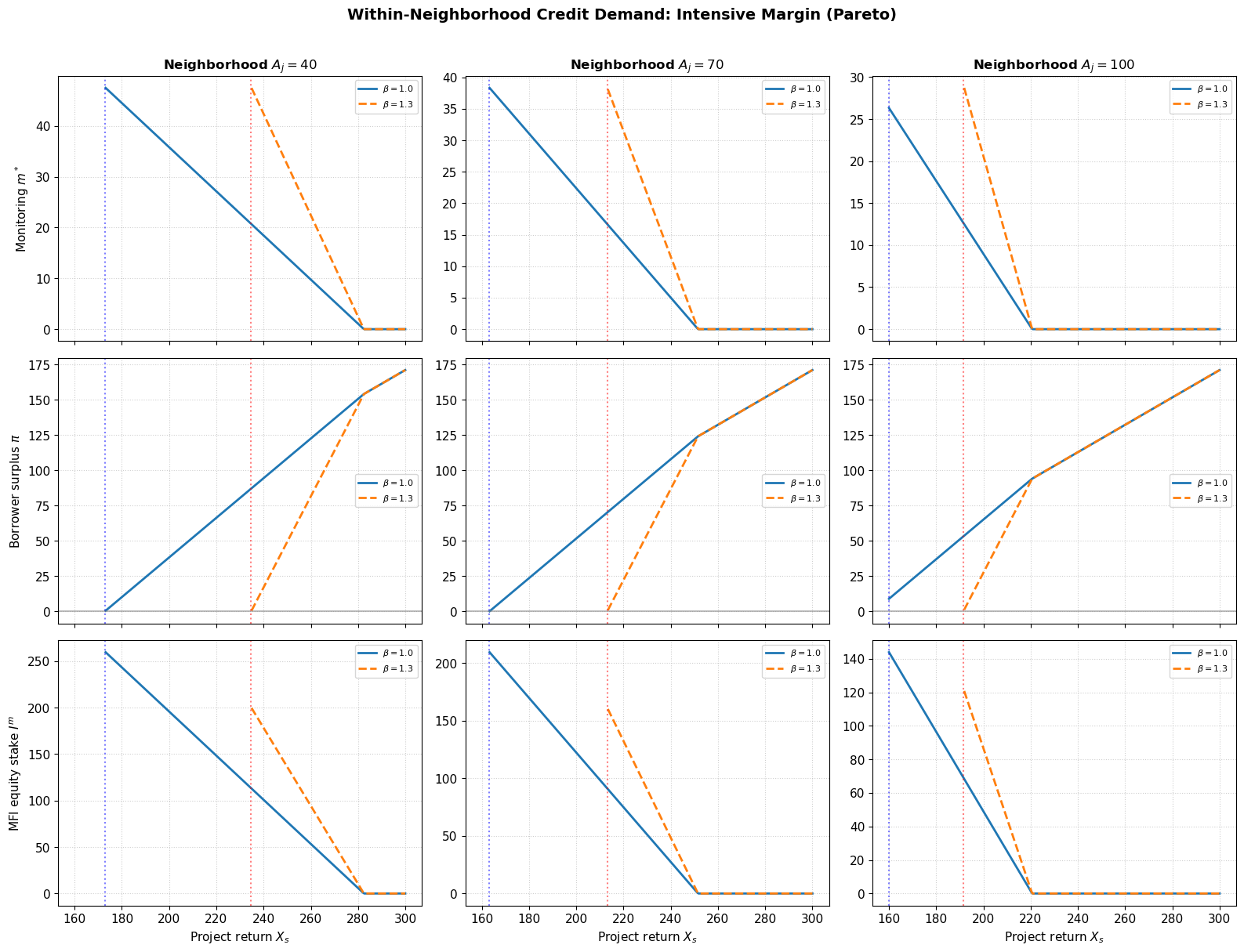
4. The Outreach Landscape with Heterogeneous Projects
Now we can compute the outreach landscape across neighborhoods. For each neighborhood , we compute:
Fraction served — what share of the local population gets credit
Total equity demanded — how much monitoring capital is absorbed
Total borrower surplus — welfare generated
We compare the social benchmark () with a range of commercial hurdle rates.
Source
# Outreach landscape across neighborhoods for different beta

A_nbhds = np.linspace(5, 140, 100)
betas_compare = [1.0, 1.1, 1.2, 1.3, 1.5]
colors_beta = cm.coolwarm(np.linspace(0.0, 1.0, len(betas_compare)))

fig, axes = plt.subplots(2, 2, figsize=(15, 11))

for beta_v, color in zip(betas_compare, colors_beta):
    frac_served_vals = []
    N_served_vals = []
    K_demand_vals = []
    total_surplus_vals = []
    X_star_vals = []

    for A_j in A_nbhds:
        bank = BankHetX(np.array([A_j]), beta=beta_v, dist_type='pareto', X_m=160, alpha_pareto=3.0)
        frac_served_vals.append(bank.frac_served(A_j))
        N_served_vals.append(bank.N_served(A_j))
        K_demand_vals.append(bank.K_demand_nbhd(A_j))
        total_surplus_vals.append(bank.total_surplus_nbhd(A_j))
        X_star_vals.append(bank.X_star(A_j))

    lbl = rf'$\beta = {beta_v:.1f}$'

    axes[0, 0].plot(A_nbhds, frac_served_vals, color=color, linewidth=2, label=lbl)
    axes[0, 1].plot(A_nbhds, X_star_vals, color=color, linewidth=2, label=lbl)
    axes[1, 0].plot(A_nbhds, K_demand_vals, color=color, linewidth=2, label=lbl)
    axes[1, 1].plot(A_nbhds, total_surplus_vals, color=color, linewidth=2, label=lbl)

axes[0, 0].set_title('Fraction of Population Served', weight='bold')
axes[0, 0].set_ylabel('Fraction served')
axes[0, 0].set_ylim(0, 1.05)

axes[0, 1].set_title(r'Marginal Project Cutoff $X_s^*$', weight='bold')
axes[0, 1].set_ylabel(r'$X_s^*$')
axes[0, 1].axhline(y=160, color='grey', linestyle=':', alpha=0.5, label=r'$X_m$')
# Guided line for X_hi removed for Pareto

axes[1, 0].set_title('MFI Equity Capital Demanded per Neighborhood', weight='bold')
axes[1, 0].set_ylabel(r'$K_j$ demanded')

axes[1, 1].set_title('Total Borrower Surplus per Neighborhood', weight='bold')
axes[1, 1].set_ylabel('Total surplus')

for ax in axes.flat:
    ax.set_xlabel(r'Neighborhood collateral $A_j$')
    ax.legend(fontsize=8)
    ax.set_xlim(0, 140)

fig.suptitle('Outreach Landscape with Pareto Project Returns',
             fontsize=14, weight='bold', y=1.01)
plt.tight_layout()
plt.savefig('figs/fig-pareto-outreach-landscape.png', dpi=300, bbox_inches='tight')
plt.show()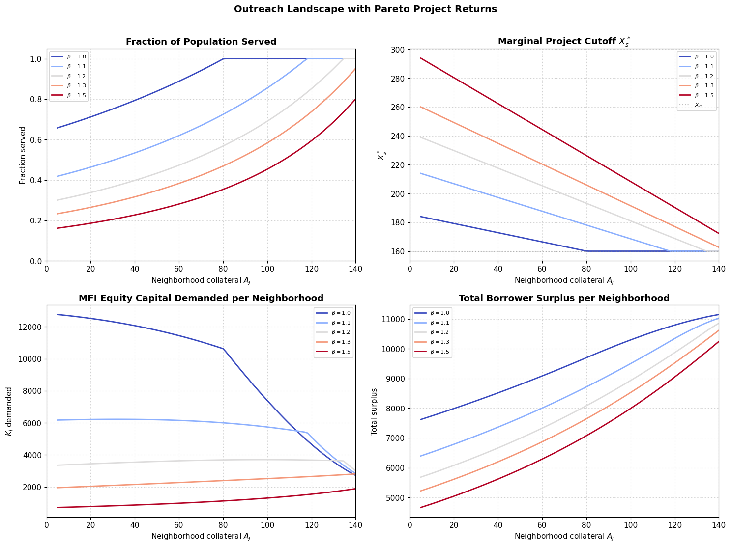
5. General Equilibrium: Clearing the Capital Market
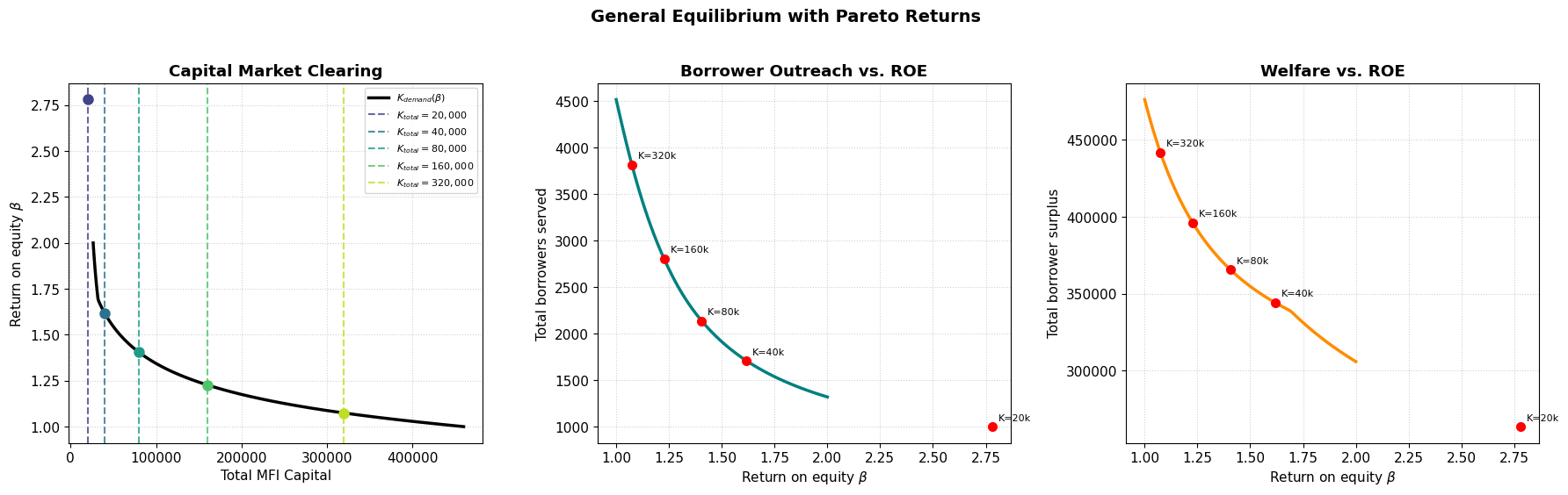
Now we close the model. Total intermediary capital is fixed in the economy. Informed equity flows to the neighborhoods offering the highest return. In equilibrium, the rate of return equalizes across all served neighborhoods.
The aggregate capital demand is:
where is the equity absorbed by neighborhood . This is a smooth, decreasing function of because:
Higher raises the monitoring cost, reducing thresholds
Fewer borrowers are served, and each absorbs different equity
We solve for the equilibrium.
Source
def total_capital_demand(beta, A_nbhds, N_pop=100, X_m=160, alpha_pareto=3.0):
    """Aggregate capital demand across all neighborhoods for Pareto."""
    bank = BankHetX(A_nbhds, beta=beta, dist_type='pareto', X_m=X_m, alpha_pareto=alpha_pareto, N_pop=N_pop)
    return bank.capital_demand_grid(A_nbhds, N_potential=N_pop)


def total_borrowers_served(beta, A_nbhds, N_pop=100, X_m=160, alpha_pareto=3.0):
    """Total borrowers served across all neighborhoods for Pareto."""
    total = 0.0
    for A_j in A_nbhds:
        bank = BankHetX(np.array([A_j]), beta=beta, dist_type='pareto', X_m=X_m, alpha_pareto=alpha_pareto, N_pop=N_pop)
        total += bank.N_served(A_j)
    return total


def total_surplus(beta, A_nbhds, N_pop=100, X_m=160, alpha_pareto=3.0):
    """Total borrower surplus across all neighborhoods for Pareto."""
    total = 0.0
    for A_j in A_nbhds:
        bank = BankHetX(np.array([A_j]), beta=beta, dist_type='pareto', X_m=X_m, alpha_pareto=alpha_pareto, N_pop=N_pop)
        total += bank.total_surplus_nbhd(A_j)
    return total


# ---- Compute K_demand schedule ----
A_nbhds_eq = np.linspace(10, 140, 50)  # 50 neighborhoods
N_pop = 100  # borrowers per neighborhood

beta_range = np.linspace(1.0, 2.0, 80)
Kd_schedule = [total_capital_demand(b, A_nbhds_eq, N_pop) for b in beta_range]
N_schedule = [total_borrowers_served(b, A_nbhds_eq, N_pop) for b in beta_range]
S_schedule = [total_surplus(b, A_nbhds_eq, N_pop) for b in beta_range]

print(f"K_demand range: [{min(Kd_schedule):.0f}, {max(Kd_schedule):.0f}]")
print(f"N_served range: [{min(N_schedule):.0f}, {max(N_schedule):.0f}]")
print(f"Surplus range:  [{min(S_schedule):.0f}, {max(S_schedule):.0f}]")
K_demand range: [26382, 459881]
N_served range: [1319, 4517]
Surplus range: [305953, 476131]
Source
K_totals = [20000, 40000, 80000, 160000, 320000]
equilibria = {}

print("=== General Equilibrium under Pareto Returns ===")
for K_tot in K_totals:
    try:
        b_star = BankHetX.solve_equilibrium(A_nbhds_eq, K_tot, N_potential=N_pop, dist_type='pareto', X_m=160, alpha_pareto=3.0)
        n_tot = total_borrowers_served(b_star, A_nbhds_eq, N_pop)
        s_tot = total_surplus(b_star, A_nbhds_eq, N_pop)
        equilibria[K_tot] = {'beta': b_star, 'N': n_tot, 'surplus': s_tot}
        print(f"K_total = {K_tot:7,}: beta* = {b_star:.4f}, N_total = {n_tot:.0f}, Total Surplus = {s_tot:.0f}")
    except ValueError as e:
        print(f"K_total = {K_tot:7,}: collapsed ({e})")
=== General Equilibrium under Pareto Returns ===
K_total =  20,000: beta* = 2.7802, N_total = 1000, Total Surplus = 263717
K_total =  40,000: beta* = 1.6168, N_total = 1709, Total Surplus = 344336
K_total =  80,000: beta* = 1.4047, N_total = 2137, Total Surplus = 365818
K_total = 160,000: beta* = 1.2269, N_total = 2805, Total Surplus = 396230
K_total = 320,000: beta* = 1.0742, N_total = 3817, Total Surplus = 441866
Source
# ---- Visualization: Capital Market Clearing ----

fig, axes = plt.subplots(1, 3, figsize=(18, 5.5))

# Plot 1: K_demand(beta) with K_total lines
ax = axes[0]
ax.plot(Kd_schedule, beta_range, 'k-', linewidth=2.5, label='$K_{demand}(\\beta)$')
for K_tot, color in zip(K_totals, cm.viridis(np.linspace(0.2, 0.9, len(K_totals)))):
    ax.axvline(x=K_tot, color=color, linestyle='--', alpha=0.8, label=f'$K_{{total}}={K_tot:,}$')
    if K_tot in equilibria:
        b = equilibria[K_tot]['beta']
        ax.plot(K_tot, b, 'o', color=color, markersize=8)
ax.set_xlabel('Total MFI Capital')
ax.set_ylabel(r'Return on equity $\beta$')
ax.set_title('Capital Market Clearing', weight='bold')
ax.legend(fontsize=8)

# Plot 2: N_served(beta)
ax = axes[1]
ax.plot(beta_range, N_schedule, 'teal', linewidth=2.5)
for K_tot in K_totals:
    if K_tot in equilibria:
        b = equilibria[K_tot]['beta']
        n = equilibria[K_tot]['N']
        ax.plot(b, n, 'ro', markersize=7)
        ax.annotate(f'K={K_tot//1000}k', (b, n), textcoords='offset points',
                   xytext=(5, 5), fontsize=8)
ax.set_xlabel(r'Return on equity $\beta$')
ax.set_ylabel('Total borrowers served')
ax.set_title('Borrower Outreach vs. ROE', weight='bold')

# Plot 3: Surplus(beta)
ax = axes[2]
ax.plot(beta_range, S_schedule, 'darkorange', linewidth=2.5)
for K_tot in K_totals:
    if K_tot in equilibria:
        b = equilibria[K_tot]['beta']
        s = equilibria[K_tot]['surplus']
        ax.plot(b, s, 'ro', markersize=7)
        ax.annotate(f'K={K_tot//1000}k', (b, s), textcoords='offset points',
                   xytext=(5, 5), fontsize=8)
        ax.set_xlabel(r'Return on equity $\beta$')
ax.set_ylabel('Total borrower surplus')
ax.set_title('Welfare vs. ROE', weight='bold')

plt.suptitle('General Equilibrium with Pareto Returns',
             fontsize=14, weight='bold', y=1.02)
plt.tight_layout()
plt.savefig('figs/fig-GE-clearing-hetX.png', dpi=300, bbox_inches='tight')
6. Depth vs. Breadth: The Two-Margin Decomposition
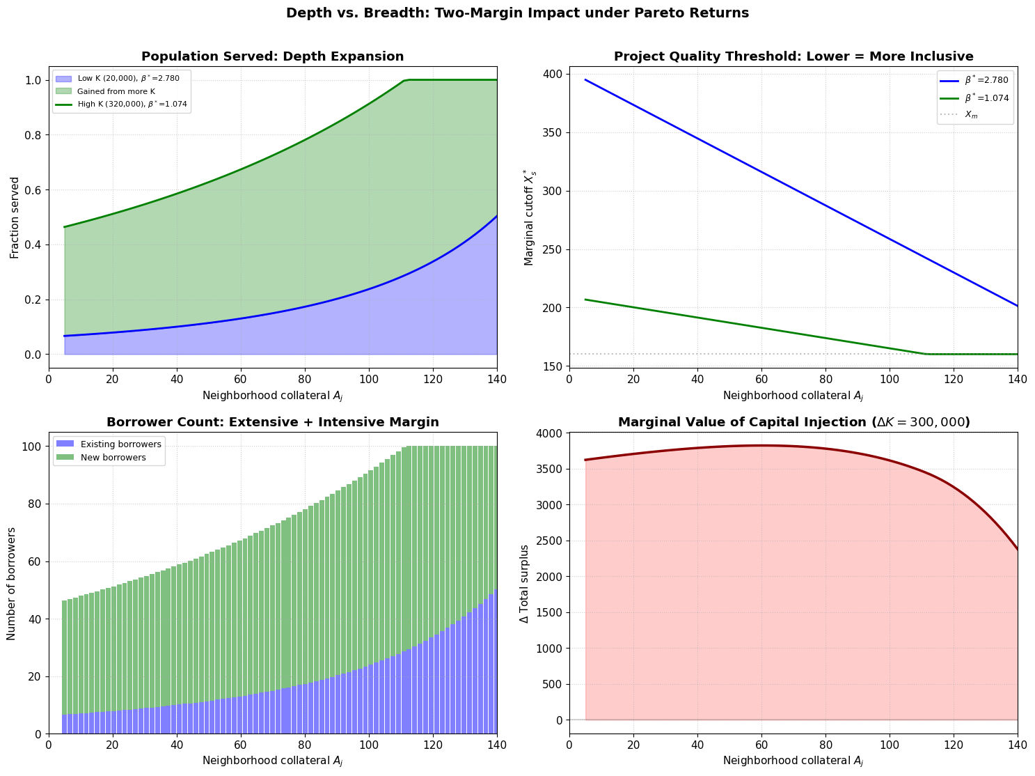
A key new result: when we inject additional capital into the economy, lending expands on two margins simultaneously:
Extensive margin (breadth): New neighborhoods become served that were previously excluded
Intensive margin (depth): Within already-served neighborhoods, more marginal borrowers (lower ) now qualify
Let’s decompose the impact of a capital increase by comparing the equilibrium allocation across neighborhoods at different levels.
Source
# Depth vs Breadth decomposition: compare two equilibria
# Pick two K_total values that have interior equilibria

K_low = None
K_high = None
for K in sorted(equilibria.keys()):
    if equilibria[K]['beta'] > 1.0:
        if K_low is None:
            K_low = K
        else:
            K_high = K

if K_low is None or K_high is None:
    # Fallback: just pick two
    K_candidates = sorted([k for k, v in equilibria.items() if v['beta'] > 1.0])
    if len(K_candidates) >= 2:
        K_low, K_high = K_candidates[0], K_candidates[-1]
    else:
        print("Need at least two interior equilibria. Adjusting K_totals...")
        K_low, K_high = 10000, 40000

print(f"Comparing K_total = {K_low} vs {K_high}")

beta_low = equilibria[K_low]['beta'] if K_low in equilibria else 1.5
beta_high = equilibria[K_high]['beta'] if K_high in equilibria else 1.1

# Compute neighborhood-level allocations for both equilibria
A_fine = np.linspace(5, 140, 80)

data_low = {'frac': [], 'N': [], 'K': [], 'surplus': [], 'Xstar': []}
data_high = {'frac': [], 'N': [], 'K': [], 'surplus': [], 'Xstar': []}

for A_j in A_fine:
    for beta_v, data in [(beta_low, data_low), (beta_high, data_high)]:
        bank = BankHetX(np.array([A_j]), beta=beta_v, dist_type='pareto', X_m=160, alpha_pareto=3.0, N_pop=N_pop)
        data['frac'].append(bank.frac_served(A_j))
        data['N'].append(bank.N_served(A_j))
        data['K'].append(bank.K_demand_nbhd(A_j))
        data['surplus'].append(bank.total_surplus_nbhd(A_j))
        data['Xstar'].append(bank.X_star(A_j))

# Convert to arrays
for d in [data_low, data_high]:
    for k in d:
        d[k] = np.array(d[k])

# Plot the decomposition
fig, axes = plt.subplots(2, 2, figsize=(15, 11))

ax = axes[0, 0]
ax.fill_between(A_fine, 0, data_low['frac'], alpha=0.3, color='blue',
                label=f'Low K ({K_low:,}), $\\beta^*$={beta_low:.3f}')
ax.fill_between(A_fine, data_low['frac'], data_high['frac'], alpha=0.3, color='green',
                label=f'Gained from more K')
ax.plot(A_fine, data_high['frac'], 'g-', linewidth=2,
        label=f'High K ({K_high:,}), $\\beta^*$={beta_high:.3f}')
ax.plot(A_fine, data_low['frac'], 'b-', linewidth=2)
ax.set_ylabel('Fraction served')
ax.set_title('Population Served: Depth Expansion', weight='bold')
ax.legend(fontsize=8)

ax = axes[0, 1]
ax.plot(A_fine, data_low['Xstar'], 'b-', linewidth=2, label=f'$\\beta^*$={beta_low:.3f}')
ax.plot(A_fine, data_high['Xstar'], 'g-', linewidth=2, label=f'$\\beta^*$={beta_high:.3f}')
ax.axhline(y=160, color='grey', linestyle=':', alpha=0.5, label=r'$X_m$')
# Guided line for X_hi removed for Pareto
ax.set_ylabel('Marginal cutoff $X_s^*$')
ax.set_title('Project Quality Threshold: Lower = More Inclusive', weight='bold')
ax.legend(fontsize=9)

ax = axes[1, 0]
delta_N = data_high['N'] - data_low['N']
ax.bar(A_fine, data_low['N'], width=1.5, color='blue', alpha=0.5, label='Existing borrowers')
ax.bar(A_fine, delta_N, width=1.5, bottom=data_low['N'], color='green', alpha=0.5, label='New borrowers')
ax.set_ylabel('Number of borrowers')
ax.set_title('Borrower Count: Extensive + Intensive Margin', weight='bold')
ax.legend(fontsize=9)

ax = axes[1, 1]
delta_S = data_high['surplus'] - data_low['surplus']
ax.plot(A_fine, delta_S, 'darkred', linewidth=2.5)
ax.fill_between(A_fine, 0, delta_S, alpha=0.2, color='red')
ax.set_ylabel('$\\Delta$ Total surplus')
ax.set_title(f'Marginal Value of Capital Injection ($\\Delta K = {K_high - K_low:,}$)', weight='bold')
ax.axhline(y=0, color='grey', linestyle='-', alpha=0.3)

for ax in axes.flat:
    ax.set_xlabel('Neighborhood collateral $A_j$')
    ax.set_xlim(0, 140)

fig.suptitle('Depth vs. Breadth: Two-Margin Impact under Pareto Returns',
             fontsize=14, weight='bold', y=1.01)
plt.tight_layout()
plt.savefig('figs/fig-depth-vs-breadth-pareto.png', dpi=300, bbox_inches='tight')
plt.show()
Comparing K_total = 20000 vs 320000
7. Mission Drift Under Commercial Pressure
One of the most important implications of this model is a precise formalization of mission drift. When the return on equity rises (e.g., because a social MFI is taken over by commercial investors, or because the overall capital supply shrinks):
Cream-skimming within neighborhoods: rises, so only the best projects within each neighborhood get funded
Neighborhood abandonment: Poorer neighborhoods with low become entirely unserved
Capital reallocation: Equity migrates from poor to rich neighborhoods
Let’s visualize this “mission drift” as increases from the social benchmark to a fully commercial level.
Source
# Mission drift visualization: heatmap of service coverage under Pareto
beta_mission = np.linspace(1.0, 1.8, 50)
A_mission = np.linspace(5, 140, 60)

frac_matrix = np.zeros((len(beta_mission), len(A_mission)))
K_matrix = np.zeros_like(frac_matrix)

for i, b in enumerate(beta_mission):
    for j, A_j in enumerate(A_mission):
        bank = BankHetX(np.array([A_j]), beta=b, dist_type='pareto', X_m=160, alpha_pareto=3.0, N_pop=N_pop)
        frac_matrix[i, j] = bank.frac_served(A_j)
        K_matrix[i, j] = bank.K_demand_nbhd(A_j)

fig, axes = plt.subplots(1, 2, figsize=(16, 6))

# Heatmap 1: Fraction served
im1 = axes[0].imshow(frac_matrix, aspect='auto', origin='lower',
                     extent=[A_mission[0], A_mission[-1], beta_mission[0], beta_mission[-1]],
                     cmap='YlGnBu', vmin=0, vmax=1)
axes[0].set_xlabel('Neighborhood collateral $A_j$', fontsize=11)
axes[0].set_ylabel(r'Return on equity $\beta$', fontsize=11)
axes[0].set_title('Fraction of Population Served (Pareto)', weight='bold', fontsize=12)
fig.colorbar(im1, ax=axes[0], label='Fraction served', shrink=0.8)

# Mark equilibria
for K_tot, eq in sorted(equilibria.items()):
    if eq['beta'] > 1.0:
        axes[0].axhline(y=eq['beta'], color='red', linestyle='--', alpha=0.5)
        axes[0].text(A_mission[-1]+2, eq['beta'], f"K={K_tot//1000}k", fontsize=8,
                    va='center', color='red')

# Heatmap 2: Capital allocated
im2 = axes[1].imshow(K_matrix, aspect='auto', origin='lower',
                     extent=[A_mission[0], A_mission[-1], beta_mission[0], beta_mission[-1]],
                     cmap='YlOrRd')
axes[1].set_xlabel('Neighborhood collateral $A_j$', fontsize=11)
axes[1].set_ylabel(r'Return on equity $\beta$', fontsize=11)
axes[1].set_title('MFI Equity Capital per Neighborhood (Pareto)', weight='bold', fontsize=12)
fig.colorbar(im2, ax=axes[1], label='$K_j$ demanded', shrink=0.8)

fig.suptitle('Mission Drift: How Pareto Returns Concentrate Commercial Capital',
             fontsize=14, weight='bold', y=1.02)
plt.tight_layout()
plt.savefig('figs/fig-mission-drift-heatmap-pareto.png', dpi=300, bbox_inches='tight')
plt.show()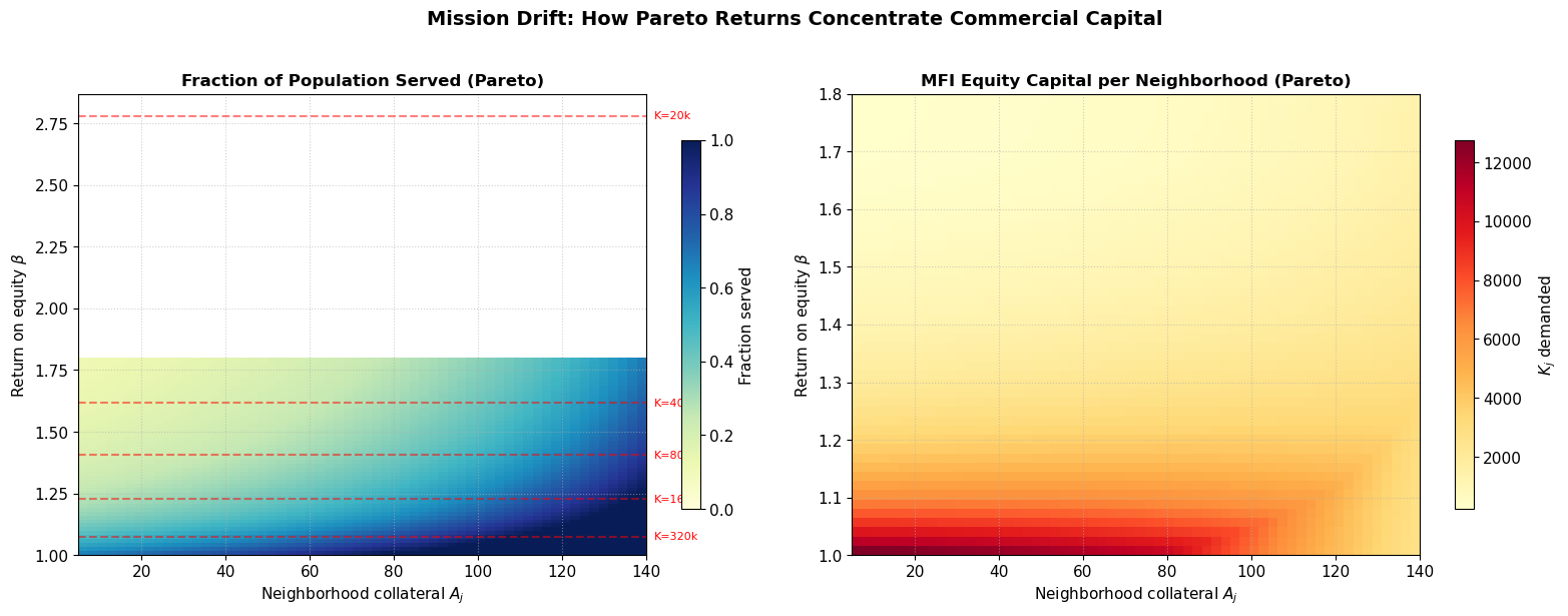
8. Social Investor Impact: Targeted vs. Untargeted Capital Injection
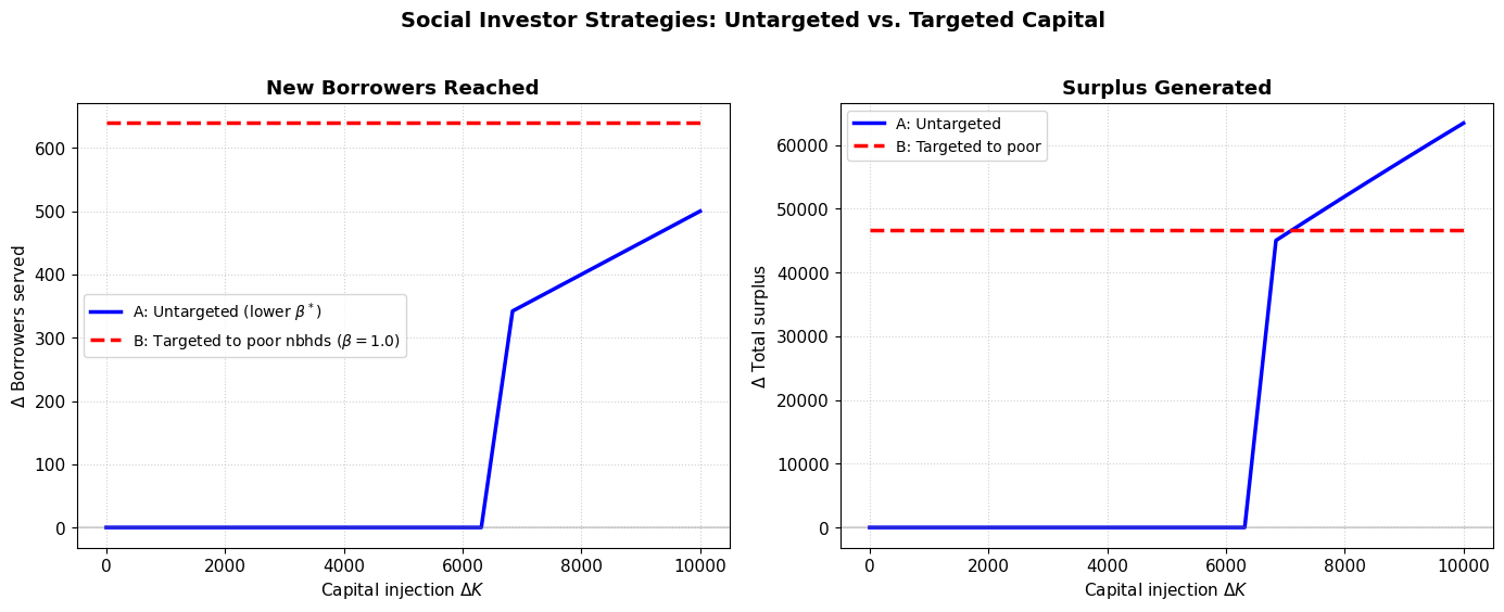
Suppose a social investor has of capital to inject into the economy. Two strategies:
Strategy A (Untargeted): Add to the general pool. This lowers economy-wide, benefiting all neighborhoods.
Strategy B (Targeted to poor neighborhoods): Inject as concessional equity () in specific poor neighborhoods. This directly expands access there without changing elsewhere.
Let’s compare the total impact (borrowers reached, surplus generated) of each strategy.
Source
# Social investor impact analysis
# Pick a baseline K_total and compute a reference equilibrium

# Use the middle K_total as baseline
K_baseline = sorted([k for k, v in equilibria.items() if v['beta'] > 1.01])[0]
beta_baseline = equilibria[K_baseline]['beta']
N_baseline = equilibria[K_baseline]['N']
S_baseline = equilibria[K_baseline]['surplus']

print(f"Baseline: K_total = {K_baseline:,}, beta* = {beta_baseline:.4f}")
print(f"          N_total = {N_baseline:.0f}, Surplus = {S_baseline:.0f}")
print()

# Inject amounts
delta_Ks = np.linspace(0, K_baseline * 0.5, 20)

# Strategy A: Untargeted (increase K_total)
results_A = {'N': [], 'S': [], 'beta': []}
for dK in delta_Ks:
    K_new = K_baseline + dK
    try:
        kd_at_1 = total_capital_demand(1.0, A_nbhds_eq, N_pop)
        if K_new >= kd_at_1:
            b = 1.0
        else:
            b = brentq(lambda beta: total_capital_demand(beta, A_nbhds_eq, N_pop) - K_new,
                       1.0, 2.0)
    except:
        b = beta_baseline
    results_A['beta'].append(b)
    results_A['N'].append(total_borrowers_served(b, A_nbhds_eq, N_pop))
    results_A['S'].append(total_surplus(b, A_nbhds_eq, N_pop))

# Strategy B: Targeted to poorest 10 neighborhoods at beta=1.0 (social equity)
# The rest of the economy still clears at beta*
# Approximate: in poor neighborhoods, use beta=1.0; elsewhere, beta = beta_baseline
results_B = {'N': [], 'S': []}
A_poor = A_nbhds_eq[:10]  # poorest 10 neighborhoods
A_rest = A_nbhds_eq[10:]  # remaining neighborhoods

for dK in delta_Ks:
    # Poor neighborhoods get subsidized equity at beta=1.0
    N_poor = 0
    S_poor = 0
    for A_j in A_poor:
        bank = BankHetX(np.array([A_j]), beta=1.0, dist_type='pareto', X_m=160, alpha_pareto=3.0, N_pop=N_pop)
        N_poor += bank.N_served(A_j)
        S_poor += bank.total_surplus_nbhd(A_j)

    # Rest of economy at beta_baseline (unchanged)
    N_rest = 0
    S_rest = 0
    for A_j in A_rest:
        bank = BankHetX(np.array([A_j]), beta=beta_baseline, dist_type='pareto', X_m=160, alpha_pareto=3.0, N_pop=N_pop)
        N_rest += bank.N_served(A_j)
        S_rest += bank.total_surplus_nbhd(A_j)

    results_B['N'].append(N_poor + N_rest)
    results_B['S'].append(S_poor + S_rest)

# Plot comparison
fig, axes = plt.subplots(1, 2, figsize=(14, 5.5))

ax = axes[0]
ax.plot(delta_Ks, np.array(results_A['N']) - N_baseline, 'b-', linewidth=2.5,
        label='A: Untargeted (lower $\\beta^*$)')
ax.plot(delta_Ks, np.array(results_B['N']) - N_baseline, 'r--', linewidth=2.5,
        label='B: Targeted to poor nbhds ($\\beta=1.0$)')
ax.set_xlabel('Capital injection $\\Delta K$')
ax.set_ylabel('$\\Delta$ Borrowers served')
ax.set_title('New Borrowers Reached', weight='bold')
ax.legend(fontsize=10)
ax.axhline(y=0, color='grey', linestyle='-', alpha=0.3)

ax = axes[1]
ax.plot(delta_Ks, np.array(results_A['S']) - S_baseline, 'b-', linewidth=2.5,
        label='A: Untargeted')
ax.plot(delta_Ks, np.array(results_B['S']) - S_baseline, 'r--', linewidth=2.5,
        label='B: Targeted to poor')
ax.set_xlabel('Capital injection $\\Delta K$')
ax.set_ylabel('$\\Delta$ Total surplus')
ax.set_title('Surplus Generated', weight='bold')
ax.legend(fontsize=10)
ax.axhline(y=0, color='grey', linestyle='-', alpha=0.3)

fig.suptitle('Social Investor Strategies: Untargeted vs. Targeted Capital',
             fontsize=14, weight='bold', y=1.02)
plt.tight_layout()
plt.savefig('figs/fig-social-investor-strategies-pareto.png', dpi=300, bbox_inches='tight')
plt.show()
Baseline: K_total = 20,000, beta* = 2.7802
N_total = 1000, Surplus = 263717
9. Analytical Results: Closed-Form Expressions
Proposition: Marginal Project Cutoff
For a neighborhood with collateral and a uniform distribution , the marginal project cutoff under leveraged lending with equity return is:
where:
is the monitoring sensitivity
is the effective monitoring cost multiplier
Comparative Statics
Proposition: and .
Higher raises the cutoff: cream-skimming intensifies under commercial pressure
Higher lowers the cutoff: richer neighborhoods can fund more marginal projects
Fraction Served
Under the uniform distribution:
Total Capital Demand (Analytical)
For the leveraged regime, . Since is linear in , the integral over the uniform distribution has a closed form:
where is the threshold above which no monitoring is needed.
Let’s verify these analytical expressions against our numerical integration.
Source
# Compare analytical vs numerical for several (A_j, beta) pairs using Pareto returns
print("=== Verification: Analytical vs Numerical K_demand (Pareto) ===")
print(f"{'A_j':>6} {'beta':>6} {'K_numerical':>12} {'K_analytical':>14} {'Match':>8}")
print("-" * 50)

for A_j in [30, 60, 90, 120]:
    for beta_v in [1.0, 1.2, 1.5]:
        bank = BankHetX(np.array([A_j]), beta=beta_v, dist_type='pareto', X_m=160, alpha_pareto=3.0, N_pop=N_pop)
        K_num = bank.K_demand_nbhd(A_j, method='numerical')
        K_ana = bank.K_demand_nbhd(A_j, method='analytical')
        match = abs(K_num - K_ana) < 0.1 * max(K_num, 1.0)
        print(f"{A_j:>6} {beta_v:>6.1f} {K_num:>12.2f} {K_ana:>14.2f} {'OK' if match else 'DIFF':>8}")
=== Verification: Analytical vs Numerical K_demand (Pareto) ===
A_j beta K_numerical K_analytical Match
--------------------------------------------------
30 1.0 12309.12 12309.12 OK
30 1.2 3493.48 3493.48 OK
30 1.5 817.75 817.75 OK
60 1.0 11442.15 11442.15 OK
60 1.2 3627.42 3627.42 OK
60 1.5 979.33 979.33 OK
90 1.0 8964.36 8964.36 OK
90 1.2 3696.29 3696.29 OK
90 1.5 1204.67 1204.67 OK
120 1.0 4659.25 4659.25 OK
120 1.2 3672.51 3672.51 OK
120 1.5 1543.52 1543.52 OK
10. Effect of Pareto Shape Parameter ()
Let’s analyze how the Pareto shape parameter (which controls the skewness and tail weight of project quality) affects the general equilibrium. A higher means the tail of high-quality projects is even thinner, and borrowers are more heavily clustered near the lower bound .
Source
# ---- Experiment: Varying Pareto Shape Parameter (alpha) ----
alphas = [2.0, 2.5, 3.0, 3.5, 4.0]
K_eq = 80000.0

print(f"{'Alpha':>8} {'beta*':>8} {'N_total':>10} {'Surplus':>10}")
print("-" * 42)

results_alpha = []
for a in alphas:
    try:
        b_star = BankHetX.solve_equilibrium(A_nbhds_eq, K_eq, N_potential=N_pop, dist_type='pareto', X_m=160, alpha_pareto=a)
        n_tot = total_borrowers_served(b_star, A_nbhds_eq, N_pop, X_m=160, alpha_pareto=a)
        s_tot = total_surplus(b_star, A_nbhds_eq, N_pop, X_m=160, alpha_pareto=a)
        results_alpha.append({'alpha': a, 'beta': b_star, 'N': n_tot, 'surplus': s_tot})
        print(f"{a:>8.1f} {b_star:>8.4f} {n_tot:>10.0f} {s_tot:>10.0f}")
    except ValueError:
        print(f"{a:>8.1f} collapsed")
   Alpha    beta*    N_total    Surplus
------------------------------------------
     2.0   1.4536       2668     781865
     2.5   1.4270       2375     506809
     3.0   1.4047       2137     365818
     3.5   1.3852       1944     280044
     4.0   1.3676       1786     222698
11. Summary and Conclusions
What We’ve Shown
Within-neighborhood heterogeneity in project returns creates a smooth intensive margin: The MFI optimally serves borrowers with , and the cutoff rises with (the return on equity) and falls with (neighborhood wealth).
Both N and K are endogenous: The number of borrowers is determined by the cutoff , and capital flows across neighborhoods seeking the highest return. The equilibrium clears both markets simultaneously.
Mission drift is formalized: An increase in causes both cream-skimming within neighborhoods (intensive margin) and abandonment of poor neighborhoods (extensive margin). This is the first formal model to capture both channels.
Donor targeting has richer tradeoffs: Untargeted capital injections lower everywhere, benefiting all neighborhoods. Targeted injections at concessional rates can directly serve excluded populations without affecting the commercial equilibrium.
Analytical tractability: The uniform distribution yields closed-form expressions for all key objects (, , ), enabling clean comparative statics propositions.
Directions for Extension
Re-introduce : Fixed entry costs create a discrete entry/exit decision per neighborhood, amplifying the extensive margin
Non-uniform distributions: Pareto or log-normal project returns would better capture empirical patterns
Endogenous : Allow the cost of uninformed capital to respond to the overall lending portfolio risk
Borrower heterogeneity in : Combine within-neighborhood and distributions for the most general model