Social Finance — Notebook 5
This notebook extends the social finance model by introducing within-neighborhood heterogeneity in project returns . In the baseline model (notebook 2) and the selfish equity extension (notebook 4), every borrower in a neighborhood had the same project return . Here we relax this assumption.
Motivation
With a distribution of project qualities within each neighborhood, the MFI faces a downward-sloping demand for credit: the best projects are funded first, and the marginal project quality declines as the MFI expands. This creates a natural intensive margin:
Number of borrowers is endogenous — determined by the marginal project cutoff
Capital is endogenous — informed equity flows across neighborhoods seeking highest return
The equilibrium jointly determines , , , and in every neighborhood
Key New Insights
Mission drift formalized: Higher causes MFIs to both drop poor neighborhoods and cream-skim within neighborhoods
Depth vs. breadth: More capital lowers , expanding on two margins
Richer donor targeting: The optimal subsidy allocation now depends on the distribution of project quality
Source
import sys
import os
import numpy as np
import matplotlib
# matplotlib.use('Agg')  # non-interactive backend for batch execution
import matplotlib.pyplot as plt
import matplotlib.cm as cm
from scipy.optimize import root_scalar, brentq
from scipy.integrate import quad

# Path configuration to find local packages
sys.path.append(os.path.abspath('..'))

# Matplotlib styling
plt.rcParams['figure.figsize'] = (8.5, 6.0)
plt.rcParams['axes.grid'] = True
plt.rcParams['grid.linestyle'] = ':'
plt.rcParams['grid.alpha'] = 0.6
plt.rcParams['font.size'] = 11

# Import the core Bank class
from socialfinance.socialfinance import Bank, BankHetX

os.makedirs('figs', exist_ok=True)
print('Imports complete.')
Imports complete.
1. Analytical Foundations
The Extended Model
We retain the baseline model from socialfinance.py with one key extension: within each neighborhood (characterized by pledgeable assets ), there is a finite population of potential borrowers. Each borrower has a project with idiosyncratic success return drawn i.i.d. from a common distribution:
The same distribution applies across all neighborhoods (neighborhoods differ only in ).
Modified Contract Equations
For a borrower in neighborhood with project return , the minimum collateral requirement under leveraged intermediation with monitoring and equity return is:
Here, the operational fixed cost per borrower is priced at the cost of debt, . This is the result of a borrower-specific Weighted Average Cost of Capital (WACC):
Economic Nuances in Fixed Cost Financing: In our new formulation, the loan fixed operational cost must always be financed out of MFI equity capital (at opportunity cost ). Thus, it carries the equity premium . This bounds maximum leverage at and resolves outreach discontinuities.
Optimal Monitoring
Inverting , the required monitoring for a borrower is:
where is the zero-monitoring collateral requirement, which is decreasing in . Higher project return means more surplus available, so less monitoring is needed.
Marginal Borrower Cutoff 
The MFI serves borrowers with , where is determined by either:
(a) Borrower participation: The marginal borrower earns zero surplus:
(b) Feasibility: , i.e., the project is rich enough that monitoring is non-negative:
The binding constraint is .
2. Validation: Recovering the Baseline
Before exploring the new model, let’s verify that BankHetX recovers the baseline when degenerates to a point mass at . We also verify the analytical formula against numerical root-finding.
Source
# --- Validation 1: Point-mass X_s = 200 should match the original Bank ---

A_test = np.array([60.0])
beta_test = 1.0

# Original Bank
bank_orig = Bank(A_test, beta=beta_test)
m_orig = bank_orig.mon(A_test)[0]
Im_orig = bank_orig.Im(m_orig)
surplus_orig = bank_orig.breturn(A_test)[0]

# BankHetX with X_s = 200 (the baseline X)
bank_het = BankHetX(A_test, beta=beta_test)
m_het = bank_het.m_opt_Xs(A_test[0], 200.0)
Im_het = bank_het.Im_Xs(m_het)
surplus_het = bank_het.borrower_surplus_Xs(A_test[0], 200.0)

print("=== Validation: BankHetX at X_s=200 vs Original Bank ===")
print(f"  Monitoring:  Original = {m_orig:.4f},  HetX = {m_het:.4f}")
print(f"  Equity I^m:  Original = {Im_orig:.4f},  HetX = {Im_het:.4f}")
print(f"  Surplus:     Original = {surplus_orig:.4f},  HetX = {surplus_het:.4f}")
print()

# --- Validation 2: X_star formula ---
print("=== Validation: X_star cutoff ===")
for A_j in [30, 60, 90, 120]:
    xs_analytical = bank_het.X_star(A_j)
    # Numerical check: find X_s where surplus = 0
    try:
        xs_numerical = brentq(lambda x: bank_het.borrower_surplus_Xs(A_j, x)
                              - 1e-10, bank_het.X_lo, bank_het.X_hi)
    except ValueError:
        xs_numerical = float('nan')
    print(f"  A_j={A_j:3d}:  X_star(analytical) = {xs_analytical:.2f},  X_star(numerical) = {xs_numerical:.2f}")
=== Validation: BankHetX at X_s=200 vs Original Bank ===
Monitoring: Original = 26.8657, HetX = 26.8657
Equity I^m: Original = 100.0000, HetX = 146.8657
Surplus: Original = 47.1343, HetX = 47.1343
=== Validation: X_star cutoff ===
A_j= 30: X_star(analytical) = 176.00, X_star(numerical) = 176.00
A_j= 60: X_star(analytical) = 166.44, X_star(numerical) = 166.44
A_j= 90: X_star(analytical) = 160.00, X_star(numerical) = nan
A_j=120: X_star(analytical) = 160.00, X_star(numerical) = nan
3. The Credit Demand Curve Within a Neighborhood
For a single neighborhood , we can now visualize the intensive margin: how the MFI’s lending expands as it dips deeper into the distribution.
For each served borrower, we plot:
Required monitoring — declining in
Borrower surplus — increasing in
MFI equity stake — declining in
The marginal borrower at the cutoff earns zero surplus and absorbs the most monitoring.
Source
# Credit demand curves for selected neighborhoods

beta_vals_to_show = [1.0, 1.3]
A_neighborhoods = [40, 70, 100]
X_grid = np.linspace(120, 280, 300)

fig, axes = plt.subplots(3, len(A_neighborhoods), figsize=(16, 12), sharex=True)

for col, A_j in enumerate(A_neighborhoods):
    for beta_v, ls, lbl_sfx in zip(beta_vals_to_show, ['-', '--'],
                                     [r'$\beta=1.0$', r'$\beta=1.3$']):
        bank = BankHetX(np.array([A_j]), beta=beta_v)
        xs = bank.X_star(A_j)

        m_vals = np.array([bank.m_opt_Xs(A_j, x) for x in X_grid])
        surplus_vals = np.array([bank.borrower_surplus_Xs(A_j, x) for x in X_grid])
        Im_vals = np.array([bank.Im_Xs(bank.m_opt_Xs(A_j, x)) for x in X_grid])

        # Zero out below X_star
        mask = X_grid >= xs

        axes[0, col].plot(X_grid[mask], m_vals[mask], ls, linewidth=2, label=lbl_sfx)
        axes[0, col].axvline(x=xs, color='red' if beta_v > 1.1 else 'blue',
                             linestyle=':', alpha=0.5)

        axes[1, col].plot(X_grid[mask], surplus_vals[mask], ls, linewidth=2, label=lbl_sfx)
        axes[1, col].axhline(y=0, color='grey', linestyle='-', alpha=0.3)
        axes[1, col].axvline(x=xs, color='red' if beta_v > 1.1 else 'blue',
                             linestyle=':', alpha=0.5)

        axes[2, col].plot(X_grid[mask], Im_vals[mask], ls, linewidth=2, label=lbl_sfx)
        axes[2, col].axvline(x=xs, color='red' if beta_v > 1.1 else 'blue',
                             linestyle=':', alpha=0.5)

    axes[0, col].set_title(f'Neighborhood $A_j = {A_j}$', fontsize=12, weight='bold')

axes[0, 0].set_ylabel('Monitoring $m^*$')
axes[1, 0].set_ylabel('Borrower surplus $\\pi$')
axes[2, 0].set_ylabel('MFI equity stake $I^m$')

for ax in axes[2, :]:
    ax.set_xlabel('Project return $X_s$')

for ax in axes.flat:
    ax.legend(fontsize=8)

fig.suptitle('Within-Neighborhood Credit Demand: Intensive Margin',
             fontsize=14, weight='bold', y=1.01)
plt.tight_layout()
plt.savefig('figs/fig-within-nbhd-demand.png', dpi=300, bbox_inches='tight')
plt.show()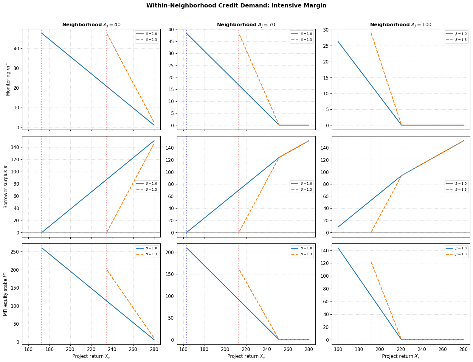
4. The Outreach Landscape with Heterogeneous Projects
Now we can compute the outreach landscape across neighborhoods. For each neighborhood , we compute:
Fraction served — what share of the local population gets credit
Total equity demanded — how much monitoring capital is absorbed
Total borrower surplus — welfare generated
We compare the social benchmark () with a range of commercial hurdle rates.
Source
# Outreach landscape across neighborhoods for different beta

A_nbhds = np.linspace(5, 140, 100)
betas_compare = [1.0, 1.1, 1.2, 1.3, 1.5]
colors_beta = cm.coolwarm(np.linspace(0.0, 1.0, len(betas_compare)))

fig, axes = plt.subplots(2, 2, figsize=(15, 11))

for beta_v, color in zip(betas_compare, colors_beta):
    frac_served_vals = []
    N_served_vals = []
    K_demand_vals = []
    total_surplus_vals = []
    X_star_vals = []

    for A_j in A_nbhds:
        bank = BankHetX(np.array([A_j]), beta=beta_v)
        frac_served_vals.append(bank.frac_served(A_j))
        N_served_vals.append(bank.N_served(A_j))
        K_demand_vals.append(bank.K_demand_nbhd(A_j))
        total_surplus_vals.append(bank.total_surplus_nbhd(A_j))
        X_star_vals.append(bank.X_star(A_j))

    lbl = rf'$\beta = {beta_v:.1f}$'

    axes[0, 0].plot(A_nbhds, frac_served_vals, color=color, linewidth=2, label=lbl)
    axes[0, 1].plot(A_nbhds, X_star_vals, color=color, linewidth=2, label=lbl)
    axes[1, 0].plot(A_nbhds, K_demand_vals, color=color, linewidth=2, label=lbl)
    axes[1, 1].plot(A_nbhds, total_surplus_vals, color=color, linewidth=2, label=lbl)

axes[0, 0].set_title('Fraction of Population Served', weight='bold')
axes[0, 0].set_ylabel('Fraction served')
axes[0, 0].set_ylim(0, 1.05)

axes[0, 1].set_title(r'Marginal Project Cutoff $X_s^*$', weight='bold')
axes[0, 1].set_ylabel(r'$X_s^*$')
axes[0, 1].axhline(y=120, color='grey', linestyle=':', alpha=0.5, label=r'$X_{lo}$')
axes[0, 1].axhline(y=280, color='grey', linestyle=':', alpha=0.5, label=r'$X_{hi}$')

axes[1, 0].set_title('MFI Equity Capital Demanded per Neighborhood', weight='bold')
axes[1, 0].set_ylabel(r'$K_j$ demanded')

axes[1, 1].set_title('Total Borrower Surplus per Neighborhood', weight='bold')
axes[1, 1].set_ylabel('Total surplus')

for ax in axes.flat:
    ax.set_xlabel(r'Neighborhood collateral $A_j$')
    ax.legend(fontsize=8)
    ax.set_xlim(0, 140)

fig.suptitle('Outreach Landscape with Heterogeneous Project Returns',
             fontsize=14, weight='bold', y=1.01)
plt.tight_layout()
plt.savefig('figs/fig-het-outreach-landscape.png', dpi=300, bbox_inches='tight')
plt.show()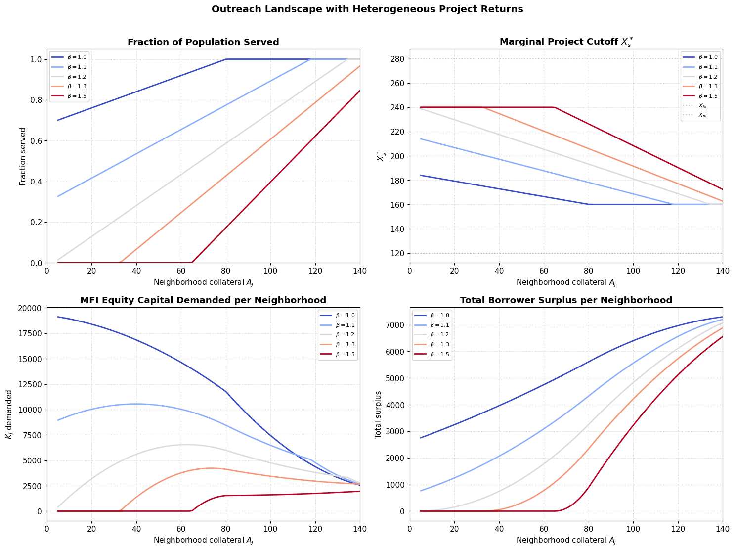
5. General Equilibrium: Clearing the Capital Market
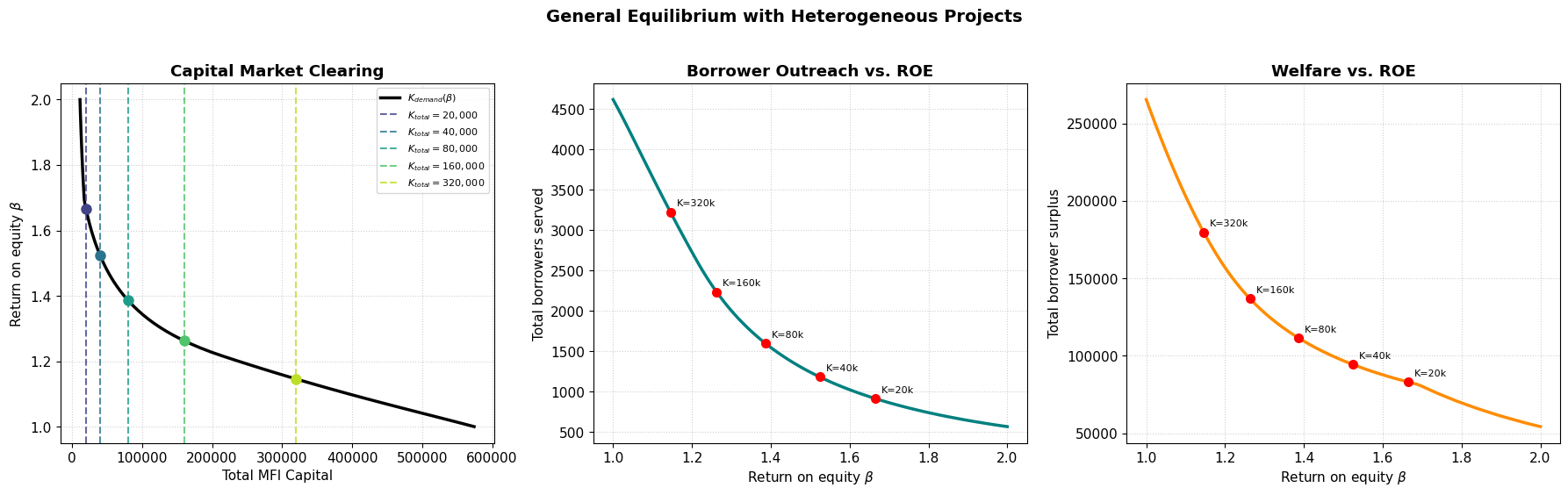
Now we close the model. Total intermediary capital is fixed in the economy. Informed equity flows to the neighborhoods offering the highest return. In equilibrium, the rate of return equalizes across all served neighborhoods.
The aggregate capital demand is:
where is the equity absorbed by neighborhood . This is a smooth, decreasing function of because:
Higher raises the monitoring cost, reducing thresholds
Fewer borrowers are served, and each absorbs different equity
We solve for the equilibrium.
Source
def total_capital_demand(beta, A_nbhds, N_pop=100, X_lo=160, X_hi=240):
    """Aggregate capital demand across all neighborhoods for a given beta."""
    bank = BankHetX(A_nbhds, beta=beta, X_lo=X_lo, X_hi=X_hi, N_pop=N_pop)
    return bank.capital_demand_grid(A_nbhds, N_potential=N_pop)


def total_borrowers_served(beta, A_nbhds, N_pop=100, X_lo=160, X_hi=240):
    """Total borrowers served across all neighborhoods for a given beta."""
    total = 0.0
    for A_j in A_nbhds:
        bank = BankHetX(np.array([A_j]), beta=beta, X_lo=X_lo, X_hi=X_hi, N_pop=N_pop)
        total += bank.N_served(A_j)
    return total


def total_surplus(beta, A_nbhds, N_pop=100, X_lo=160, X_hi=240):
    """Total borrower surplus across all neighborhoods for a given beta."""
    total = 0.0
    for A_j in A_nbhds:
        bank = BankHetX(np.array([A_j]), beta=beta, X_lo=X_lo, X_hi=X_hi, N_pop=N_pop)
        total += bank.total_surplus_nbhd(A_j)
    return total


# ---- Compute K_demand schedule ----
A_nbhds_eq = np.linspace(10, 140, 50)  # 50 neighborhoods
N_pop = 100  # borrowers per neighborhood

beta_range = np.linspace(1.0, 2.0, 80)
Kd_schedule = [total_capital_demand(b, A_nbhds_eq, N_pop) for b in beta_range]
N_schedule = [total_borrowers_served(b, A_nbhds_eq, N_pop) for b in beta_range]
S_schedule = [total_surplus(b, A_nbhds_eq, N_pop) for b in beta_range]

print(f"K_demand range: [{min(Kd_schedule):.0f}, {max(Kd_schedule):.0f}]")
print(f"N_served range: [{min(N_schedule):.0f}, {max(N_schedule):.0f}]")
K_demand range: [11367, 574316]
N_served range: [568, 4616]
Source
# ---- Solve for equilibrium at several K_total levels ----
# Choose K_total values that span a meaningful range

K_totals = [20000, 40000, 80000, 160000, 320000]
equilibria = {}

for K_tot in K_totals:
    def eq_func(beta):
        return total_capital_demand(beta, A_nbhds_eq, N_pop) - K_tot

    # Check if equilibrium exists within [1.0, 2.0]
    kd_low = total_capital_demand(1.0, A_nbhds_eq, N_pop)
    kd_high = total_capital_demand(2.0, A_nbhds_eq, N_pop)

    if K_tot > kd_low:
        print(f"K_total = {K_tot:>6}: Capital oversupply (K_demand at beta=1.0 is {kd_low:.0f}). beta* = 1.0")
        equilibria[K_tot] = {'beta': 1.0, 'N': total_borrowers_served(1.0, A_nbhds_eq, N_pop),
                             'surplus': total_surplus(1.0, A_nbhds_eq, N_pop)}
    elif K_tot < kd_high:
        print(f"K_total = {K_tot:>6}: Capital too scarce (K_demand at beta=2.0 is {kd_high:.0f}). Extend range.")
    else:
        sol = brentq(eq_func, 1.0, 2.0)
        n_tot = total_borrowers_served(sol, A_nbhds_eq, N_pop)
        s_tot = total_surplus(sol, A_nbhds_eq, N_pop)
        equilibria[K_tot] = {'beta': sol, 'N': n_tot, 'surplus': s_tot}
        print(f"K_total = {K_tot:>6}: beta* = {sol:.4f}, N_total = {n_tot:.0f}, Total Surplus = {s_tot:.0f}")

print("\n--- Equilibrium Summary ---")
print(f"{'K_total':>10} {'beta*':>8} {'N_total':>10} {'Surplus':>10}")
for K, eq in sorted(equilibria.items()):
    print(f"{K:>10} {eq['beta']:>8.4f} {eq['N']:>10.0f} {eq['surplus']:>10.0f}")
K_total =  20000: beta* = 1.6650, N_total = 916, Total Surplus = 83084
K_total =  40000: beta* = 1.5242, N_total = 1183, Total Surplus = 94395
K_total =  80000: beta* = 1.3861, N_total = 1600, Total Surplus = 111568
K_total = 160000: beta* = 1.2627, N_total = 2234, Total Surplus = 137017
K_total = 320000: beta* = 1.1457, N_total = 3221, Total Surplus = 179842

--- Equilibrium Summary ---
   K_total    beta*    N_total    Surplus
     20000   1.6650        916      83084
     40000   1.5242       1183      94395
     80000   1.3861       1600     111568
    160000   1.2627       2234     137017
    320000   1.1457       3221     179842
Source
# ---- Visualization: Capital Market Clearing ----

fig, axes = plt.subplots(1, 3, figsize=(18, 5.5))

# Plot 1: K_demand(beta) with K_total lines
ax = axes[0]
ax.plot(Kd_schedule, beta_range, 'k-', linewidth=2.5, label='$K_{demand}(\\beta)$')
for K_tot, color in zip(K_totals, cm.viridis(np.linspace(0.2, 0.9, len(K_totals)))):
    ax.axvline(x=K_tot, color=color, linestyle='--', alpha=0.8, label=f'$K_{{total}}={K_tot:,}$')
    if K_tot in equilibria:
        b = equilibria[K_tot]['beta']
        ax.plot(K_tot, b, 'o', color=color, markersize=8)
ax.set_xlabel('Total MFI Capital')
ax.set_ylabel(r'Return on equity $\beta$')
ax.set_title('Capital Market Clearing', weight='bold')
ax.legend(fontsize=8)

# Plot 2: N_served(beta)
ax = axes[1]
ax.plot(beta_range, N_schedule, 'teal', linewidth=2.5)
for K_tot in K_totals:
    if K_tot in equilibria:
        b = equilibria[K_tot]['beta']
        n = equilibria[K_tot]['N']
        ax.plot(b, n, 'ro', markersize=7)
        ax.annotate(f'K={K_tot//1000}k', (b, n), textcoords='offset points',
                   xytext=(5, 5), fontsize=8)
ax.set_xlabel(r'Return on equity $\beta$')
ax.set_ylabel('Total borrowers served')
ax.set_title('Borrower Outreach vs. ROE', weight='bold')

# Plot 3: Surplus(beta)
ax = axes[2]
ax.plot(beta_range, S_schedule, 'darkorange', linewidth=2.5)
for K_tot in K_totals:
    if K_tot in equilibria:
        b = equilibria[K_tot]['beta']
        s = equilibria[K_tot]['surplus']
        ax.plot(b, s, 'ro', markersize=7)
        ax.annotate(f'K={K_tot//1000}k', (b, s), textcoords='offset points',
                   xytext=(5, 5), fontsize=8)
        ax.set_xlabel(r'Return on equity $\beta$')
ax.set_ylabel('Total borrower surplus')
ax.set_title('Welfare vs. ROE', weight='bold')

plt.suptitle('General Equilibrium with Heterogeneous Projects',
             fontsize=14, weight='bold', y=1.02)
plt.tight_layout()
plt.savefig('figs/fig-GE-clearing-hetX.png', dpi=300, bbox_inches='tight')
6. Depth vs. Breadth: The Two-Margin Decomposition
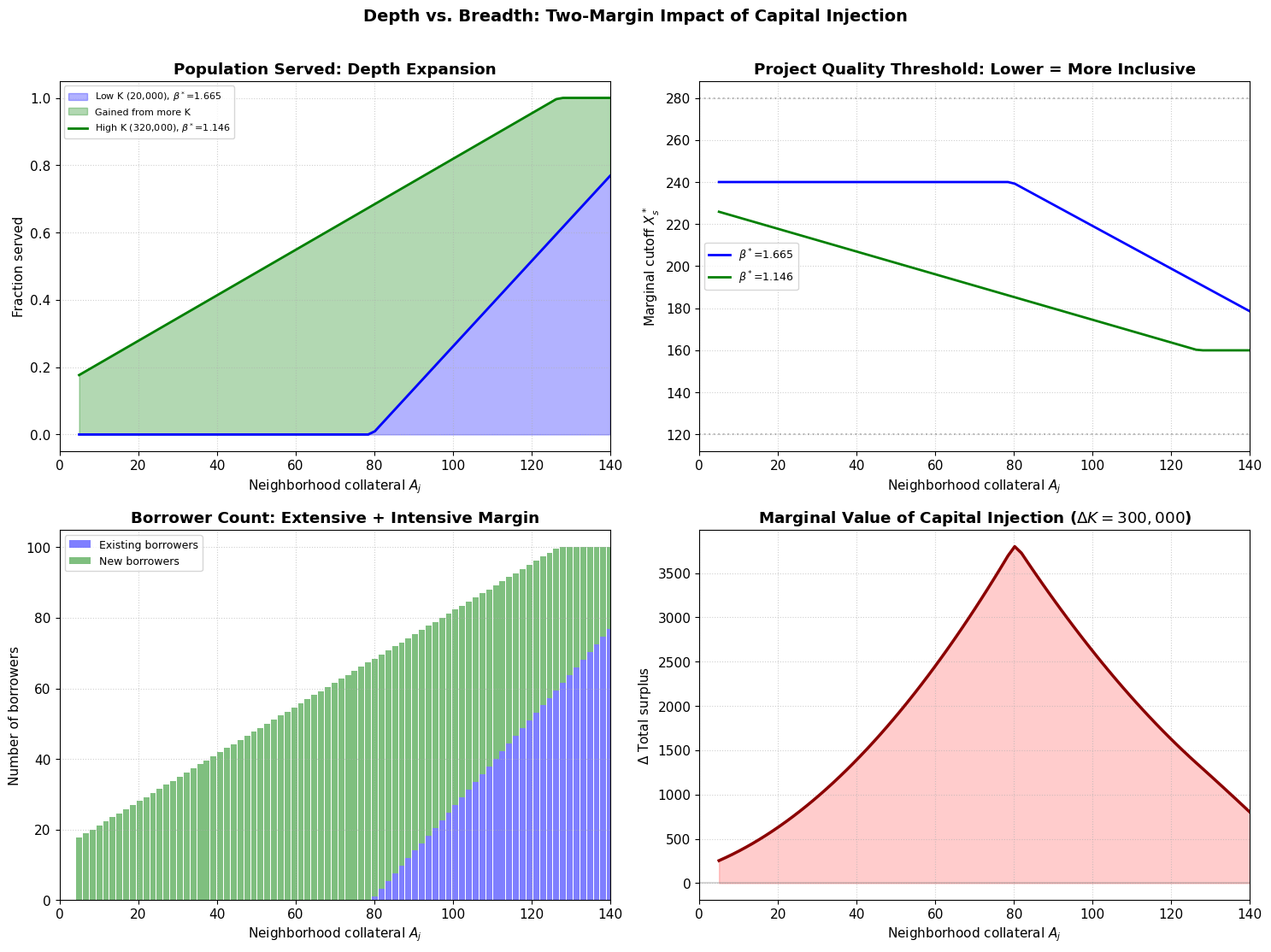
A key new result: when we inject additional capital into the economy, lending expands on two margins simultaneously:
Extensive margin (breadth): New neighborhoods become served that were previously excluded
Intensive margin (depth): Within already-served neighborhoods, more marginal borrowers (lower ) now qualify
Let’s decompose the impact of a capital increase by comparing the equilibrium allocation across neighborhoods at different levels.
Source
# Depth vs Breadth decomposition: compare two equilibria
# Pick two K_total values that have interior equilibria

K_low = None
K_high = None
for K in sorted(equilibria.keys()):
    if equilibria[K]['beta'] > 1.0:
        if K_low is None:
            K_low = K
        else:
            K_high = K

if K_low is None or K_high is None:
    # Fallback: just pick two
    K_candidates = sorted([k for k, v in equilibria.items() if v['beta'] > 1.0])
    if len(K_candidates) >= 2:
        K_low, K_high = K_candidates[0], K_candidates[-1]
    else:
        print("Need at least two interior equilibria. Adjusting K_totals...")
        K_low, K_high = 10000, 40000

print(f"Comparing K_total = {K_low} vs {K_high}")

beta_low = equilibria[K_low]['beta'] if K_low in equilibria else 1.5
beta_high = equilibria[K_high]['beta'] if K_high in equilibria else 1.1

# Compute neighborhood-level allocations for both equilibria
A_fine = np.linspace(5, 140, 80)

data_low = {'frac': [], 'N': [], 'K': [], 'surplus': [], 'Xstar': []}
data_high = {'frac': [], 'N': [], 'K': [], 'surplus': [], 'Xstar': []}

for A_j in A_fine:
    for beta_v, data in [(beta_low, data_low), (beta_high, data_high)]:
        bank = BankHetX(np.array([A_j]), beta=beta_v, N_pop=N_pop)
        data['frac'].append(bank.frac_served(A_j))
        data['N'].append(bank.N_served(A_j))
        data['K'].append(bank.K_demand_nbhd(A_j))
        data['surplus'].append(bank.total_surplus_nbhd(A_j))
        data['Xstar'].append(bank.X_star(A_j))

# Convert to arrays
for d in [data_low, data_high]:
    for k in d:
        d[k] = np.array(d[k])

# Plot the decomposition
fig, axes = plt.subplots(2, 2, figsize=(15, 11))

ax = axes[0, 0]
ax.fill_between(A_fine, 0, data_low['frac'], alpha=0.3, color='blue',
                label=f'Low K ({K_low:,}), $\\beta^*$={beta_low:.3f}')
ax.fill_between(A_fine, data_low['frac'], data_high['frac'], alpha=0.3, color='green',
                label=f'Gained from more K')
ax.plot(A_fine, data_high['frac'], 'g-', linewidth=2,
        label=f'High K ({K_high:,}), $\\beta^*$={beta_high:.3f}')
ax.plot(A_fine, data_low['frac'], 'b-', linewidth=2)
ax.set_ylabel('Fraction served')
ax.set_title('Population Served: Depth Expansion', weight='bold')
ax.legend(fontsize=8)

ax = axes[0, 1]
ax.plot(A_fine, data_low['Xstar'], 'b-', linewidth=2, label=f'$\\beta^*$={beta_low:.3f}')
ax.plot(A_fine, data_high['Xstar'], 'g-', linewidth=2, label=f'$\\beta^*$={beta_high:.3f}')
ax.axhline(y=120, color='grey', linestyle=':', alpha=0.5)
ax.axhline(y=280, color='grey', linestyle=':', alpha=0.5)
ax.set_ylabel('Marginal cutoff $X_s^*$')
ax.set_title('Project Quality Threshold: Lower = More Inclusive', weight='bold')
ax.legend(fontsize=9)

ax = axes[1, 0]
delta_N = data_high['N'] - data_low['N']
ax.bar(A_fine, data_low['N'], width=1.5, color='blue', alpha=0.5, label='Existing borrowers')
ax.bar(A_fine, delta_N, width=1.5, bottom=data_low['N'], color='green', alpha=0.5, label='New borrowers')
ax.set_ylabel('Number of borrowers')
ax.set_title('Borrower Count: Extensive + Intensive Margin', weight='bold')
ax.legend(fontsize=9)

ax = axes[1, 1]
delta_S = data_high['surplus'] - data_low['surplus']
ax.plot(A_fine, delta_S, 'darkred', linewidth=2.5)
ax.fill_between(A_fine, 0, delta_S, alpha=0.2, color='red')
ax.set_ylabel('$\\Delta$ Total surplus')
ax.set_title(f'Marginal Value of Capital Injection ($\\Delta K = {K_high - K_low:,}$)', weight='bold')
ax.axhline(y=0, color='grey', linestyle='-', alpha=0.3)

for ax in axes.flat:
    ax.set_xlabel('Neighborhood collateral $A_j$')
    ax.set_xlim(0, 140)

fig.suptitle('Depth vs. Breadth: Two-Margin Impact of Capital Injection',
             fontsize=14, weight='bold', y=1.01)
plt.tight_layout()
plt.savefig('figs/fig-depth-vs-breadth.png', dpi=300, bbox_inches='tight')
plt.show()
Comparing K_total = 20000 vs 320000
7. Mission Drift Under Commercial Pressure
One of the most important implications of this model is a precise formalization of mission drift. When the return on equity rises (e.g., because a social MFI is taken over by commercial investors, or because the overall capital supply shrinks):
Cream-skimming within neighborhoods: rises, so only the best projects within each neighborhood get funded
Neighborhood abandonment: Poorer neighborhoods with low become entirely unserved
Capital reallocation: Equity migrates from poor to rich neighborhoods
Let’s visualize this “mission drift” as increases from the social benchmark to a fully commercial level.
Source
# Mission drift visualization: heatmap of service coverage

beta_mission = np.linspace(1.0, 1.8, 50)
A_mission = np.linspace(5, 140, 60)

# Build a matrix: frac_served[beta_idx, A_idx]
frac_matrix = np.zeros((len(beta_mission), len(A_mission)))
K_matrix = np.zeros_like(frac_matrix)

for i, b in enumerate(beta_mission):
    for j, A_j in enumerate(A_mission):
        bank = BankHetX(np.array([A_j]), beta=b, N_pop=N_pop)
        frac_matrix[i, j] = bank.frac_served(A_j)
        K_matrix[i, j] = bank.K_demand_nbhd(A_j)

fig, axes = plt.subplots(1, 2, figsize=(16, 6))

# Heatmap 1: Fraction served
im1 = axes[0].imshow(frac_matrix, aspect='auto', origin='lower',
                     extent=[A_mission[0], A_mission[-1], beta_mission[0], beta_mission[-1]],
                     cmap='YlGnBu', vmin=0, vmax=1)
axes[0].set_xlabel('Neighborhood collateral $A_j$', fontsize=11)
axes[0].set_ylabel(r'Return on equity $\beta$', fontsize=11)
axes[0].set_title('Fraction of Population Served', weight='bold', fontsize=12)
fig.colorbar(im1, ax=axes[0], label='Fraction served', shrink=0.8)

# Mark equilibria
for K_tot, eq in sorted(equilibria.items()):
    if eq['beta'] > 1.0:
        axes[0].axhline(y=eq['beta'], color='red', linestyle='--', alpha=0.5)
        axes[0].text(A_mission[-1]+2, eq['beta'], f"K={K_tot//1000}k", fontsize=8,
                    va='center', color='red')

# Heatmap 2: Capital allocated
im2 = axes[1].imshow(K_matrix, aspect='auto', origin='lower',
                     extent=[A_mission[0], A_mission[-1], beta_mission[0], beta_mission[-1]],
                     cmap='YlOrRd')
axes[1].set_xlabel('Neighborhood collateral $A_j$', fontsize=11)
axes[1].set_ylabel(r'Return on equity $\beta$', fontsize=11)
axes[1].set_title('MFI Equity Capital per Neighborhood', weight='bold', fontsize=12)
fig.colorbar(im2, ax=axes[1], label='$K_j$ demanded', shrink=0.8)

fig.suptitle('Mission Drift: How Rising ROE Reshapes the Lending Landscape',
             fontsize=14, weight='bold', y=1.02)
plt.tight_layout()
plt.savefig('figs/fig-mission-drift-heatmap.png', dpi=300, bbox_inches='tight')
plt.show()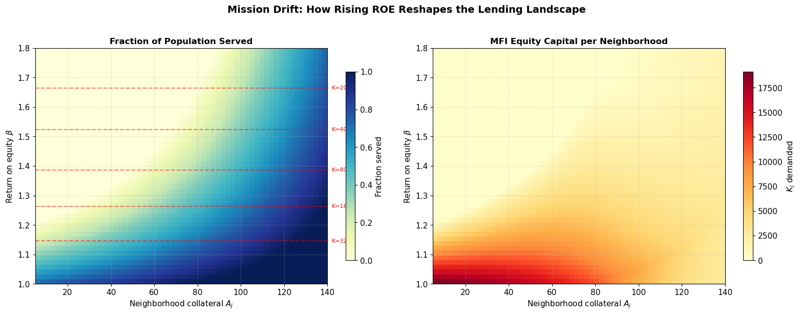
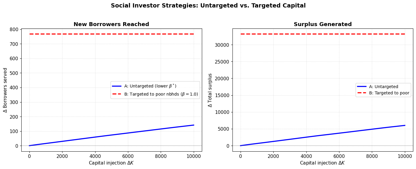
8. Social Investor Impact: Targeted vs. Untargeted Capital Injection
Suppose a social investor has of capital to inject into the economy. Two strategies:
Strategy A (Untargeted): Add to the general pool. This lowers economy-wide, benefiting all neighborhoods.
Strategy B (Targeted to poor neighborhoods): Inject as concessional equity () in specific poor neighborhoods. This directly expands access there without changing elsewhere.
Let’s compare the total impact (borrowers reached, surplus generated) of each strategy.
Source
# Social investor impact analysis
# Pick a baseline K_total and compute a reference equilibrium

# Use the middle K_total as baseline
K_baseline = sorted([k for k, v in equilibria.items() if v['beta'] > 1.01])[0]
beta_baseline = equilibria[K_baseline]['beta']
N_baseline = equilibria[K_baseline]['N']
S_baseline = equilibria[K_baseline]['surplus']

print(f"Baseline: K_total = {K_baseline:,}, beta* = {beta_baseline:.4f}")
print(f"          N_total = {N_baseline:.0f}, Surplus = {S_baseline:.0f}")
print()

# Inject amounts
delta_Ks = np.linspace(0, K_baseline * 0.5, 20)

# Strategy A: Untargeted (increase K_total)
results_A = {'N': [], 'S': [], 'beta': []}
for dK in delta_Ks:
    K_new = K_baseline + dK
    try:
        kd_at_1 = total_capital_demand(1.0, A_nbhds_eq, N_pop)
        if K_new >= kd_at_1:
            b = 1.0
        else:
            b = brentq(lambda beta: total_capital_demand(beta, A_nbhds_eq, N_pop) - K_new,
                       1.0, 2.0)
    except:
        b = beta_baseline
    results_A['beta'].append(b)
    results_A['N'].append(total_borrowers_served(b, A_nbhds_eq, N_pop))
    results_A['S'].append(total_surplus(b, A_nbhds_eq, N_pop))

# Strategy B: Targeted to poorest 10 neighborhoods at beta=1.0 (social equity)
# The rest of the economy still clears at beta*
# Approximate: in poor neighborhoods, use beta=1.0; elsewhere, beta = beta_baseline
results_B = {'N': [], 'S': []}
A_poor = A_nbhds_eq[:10]  # poorest 10 neighborhoods
A_rest = A_nbhds_eq[10:]  # remaining neighborhoods

for dK in delta_Ks:
    # Poor neighborhoods get subsidized equity at beta=1.0
    N_poor = 0
    S_poor = 0
    for A_j in A_poor:
        bank = BankHetX(np.array([A_j]), beta=1.0, N_pop=N_pop)
        N_poor += bank.N_served(A_j)
        S_poor += bank.total_surplus_nbhd(A_j)

    # Rest of economy at beta_baseline (unchanged)
    N_rest = 0
    S_rest = 0
    for A_j in A_rest:
        bank = BankHetX(np.array([A_j]), beta=beta_baseline, N_pop=N_pop)
        N_rest += bank.N_served(A_j)
        S_rest += bank.total_surplus_nbhd(A_j)

    results_B['N'].append(N_poor + N_rest)
    results_B['S'].append(S_poor + S_rest)

# Plot comparison
fig, axes = plt.subplots(1, 2, figsize=(14, 5.5))

ax = axes[0]
ax.plot(delta_Ks, np.array(results_A['N']) - N_baseline, 'b-', linewidth=2.5,
        label='A: Untargeted (lower $\\beta^*$)')
ax.plot(delta_Ks, np.array(results_B['N']) - N_baseline, 'r--', linewidth=2.5,
        label='B: Targeted to poor nbhds ($\\beta=1.0$)')
ax.set_xlabel('Capital injection $\\Delta K$')
ax.set_ylabel('$\\Delta$ Borrowers served')
ax.set_title('New Borrowers Reached', weight='bold')
ax.legend(fontsize=10)
ax.axhline(y=0, color='grey', linestyle='-', alpha=0.3)

ax = axes[1]
ax.plot(delta_Ks, np.array(results_A['S']) - S_baseline, 'b-', linewidth=2.5,
        label='A: Untargeted')
ax.plot(delta_Ks, np.array(results_B['S']) - S_baseline, 'r--', linewidth=2.5,
        label='B: Targeted to poor')
ax.set_xlabel('Capital injection $\\Delta K$')
ax.set_ylabel('$\\Delta$ Total surplus')
ax.set_title('Surplus Generated', weight='bold')
ax.legend(fontsize=10)
ax.axhline(y=0, color='grey', linestyle='-', alpha=0.3)

fig.suptitle('Social Investor Strategies: Untargeted vs. Targeted Capital',
             fontsize=14, weight='bold', y=1.02)
plt.tight_layout()
plt.savefig('figs/fig-social-investor-strategies.png', dpi=300, bbox_inches='tight')
plt.show()
Baseline: K_total = 20,000, beta* = 1.6650
N_total = 916, Surplus = 83084
9. Analytical Results: Closed-Form Expressions
Proposition: Marginal Project Cutoff
For a neighborhood with collateral and a uniform distribution , the marginal project cutoff under leveraged lending with equity return is:
where:
is the monitoring sensitivity
is the effective monitoring cost multiplier
Comparative Statics
Proposition: and .
Higher raises the cutoff: cream-skimming intensifies under commercial pressure
Higher lowers the cutoff: richer neighborhoods can fund more marginal projects
Fraction Served
Under the uniform distribution:
Total Capital Demand (Analytical)
For the leveraged regime, . Since is linear in , the integral over the uniform distribution has a closed form:
where is the threshold above which no monitoring is needed.
Let’s verify these analytical expressions against our numerical integration.
Source
# Compare analytical vs numerical for several (A_j, beta) pairs using refactored BankHetX methods
print("=== Verification: Analytical vs Numerical K_demand ===")
print(f"{'A_j':>6} {'beta':>6} {'K_numerical':>12} {'K_analytical':>14} {'Match':>8}")
print("-" * 50)

for A_j in [30, 60, 90, 120]:
    for beta_v in [1.0, 1.2, 1.5]:
        bank = BankHetX(np.array([A_j]), beta=beta_v, N_pop=N_pop)
        K_num = bank.K_demand_nbhd(A_j, method='numerical')
        K_ana = bank.K_demand_nbhd(A_j, method='analytical')
        match = abs(K_num - K_ana) < 0.1 * max(K_num, 1.0)
        print(f"{A_j:>6} {beta_v:>6.1f} {K_num:>12.2f} {K_ana:>14.2f} {'OK' if match else 'DIFF':>8}")
=== Verification: Analytical vs Numerical K_demand ===
A_j beta K_numerical K_analytical Match
--------------------------------------------------
30 1.0 17703.68 17703.68 OK
30 1.2 4574.24 4574.24 OK
30 1.5 0.00 0.00 OK
60 1.0 14641.42 14641.42 OK
60 1.2 6534.13 6534.13 OK
60 1.5 0.00 0.00 OK
90 1.0 9465.42 9465.42 OK
90 1.2 5338.23 5338.23 OK
90 1.5 1566.38 1566.38 OK
120 1.0 4374.33 4374.33 OK
120 1.2 3812.83 3812.83 OK
120 1.5 1748.16 1748.16 OK
10. Comparative Statics: How Distribution Width Affects Equilibrium
An important modeling choice is the width of the project return distribution . As the distribution collapses to a point (), we should recover the homogeneous baseline. Let’s explore how the distribution’s spread affects the equilibrium.
Source
# Effect of distribution width on equilibrium
# Keep mean fixed at 200, vary the spread

X_mean = 200
spreads = [10, 40, 80, 120, 160]  # half-width of uniform distribution
K_target = 20000

print("=== Effect of Project Return Heterogeneity ===")
print(f"{'Spread':>8} {'X_lo':>6} {'X_hi':>6} {'beta*':>8} {'N_total':>10} {'Surplus':>10}")
print("-" * 55)

results_spread = []

for spread in spreads:
    X_lo_s = X_mean - spread
    X_hi_s = X_mean + spread

    # Compute K_demand schedule for this spread
    def kd_spread(beta):
        tot = 0.0
        for A_j in A_nbhds_eq:
            bank = BankHetX(np.array([A_j]), beta=beta, X_lo=X_lo_s, X_hi=X_hi_s, N_pop=N_pop)
            tot += bank.K_demand_nbhd(A_j)
        return tot - K_target

    kd_at_1 = kd_spread(1.0) + K_target
    if K_target >= kd_at_1:
        b_star = 1.0
    else:
        try:
            b_star = brentq(kd_spread, 1.0, 3.0)
        except:
            b_star = float('nan')

    n_tot = total_borrowers_served(b_star, A_nbhds_eq, N_pop)
    # Recompute with correct X range
    n_tot = 0
    s_tot = 0
    for A_j in A_nbhds_eq:
        bank = BankHetX(np.array([A_j]), beta=b_star, X_lo=X_lo_s, X_hi=X_hi_s, N_pop=N_pop)
        n_tot += bank.N_served(A_j)
        s_tot += bank.total_surplus_nbhd(A_j)

    results_spread.append({'spread': spread, 'X_lo': X_lo_s, 'X_hi': X_hi_s,
                           'beta': b_star, 'N': n_tot, 'surplus': s_tot})
    print(f"{spread:>8} {X_lo_s:>6} {X_hi_s:>6} {b_star:>8.4f} {n_tot:>10.0f} {s_tot:>10.0f}")

print("\nKey insight: wider distribution => more cream-skimming => fewer borrowers")
print("served at equilibrium, but those served have higher average project quality.")
=== Effect of Project Return Heterogeneity ===
Spread X_lo X_hi beta* N_total Surplus
-------------------------------------------------------
10 190 210 1.6506 872 63276
40 160 240 1.6650 916 83084
80 120 280 1.8462 1000 120109
120 80 320 2.2628 1000 148932
160 40 360 2.9860 1000 177977
Key insight: wider distribution => more cream-skimming => fewer borrowers
served at equilibrium, but those served have higher average project quality.
11. Summary and Conclusions
What We’ve Shown
Within-neighborhood heterogeneity in project returns creates a smooth intensive margin: The MFI optimally serves borrowers with , and the cutoff rises with (the return on equity) and falls with (neighborhood wealth).
Both N and K are endogenous: The number of borrowers is determined by the cutoff , and capital flows across neighborhoods seeking the highest return. The equilibrium clears both markets simultaneously.
Mission drift is formalized: An increase in causes both cream-skimming within neighborhoods (intensive margin) and abandonment of poor neighborhoods (extensive margin). This is the first formal model to capture both channels.
Donor targeting has richer tradeoffs: Untargeted capital injections lower everywhere, benefiting all neighborhoods. Targeted injections at concessional rates can directly serve excluded populations without affecting the commercial equilibrium.
Analytical tractability: The uniform distribution yields closed-form expressions for all key objects (, , ), enabling clean comparative statics propositions.
Directions for Extension
Re-introduce : Fixed entry costs create a discrete entry/exit decision per neighborhood, amplifying the extensive margin
Non-uniform distributions: Pareto or log-normal project returns would better capture empirical patterns
Endogenous : Allow the cost of uninformed capital to respond to the overall lending portfolio risk
Borrower heterogeneity in : Combine within-neighborhood and distributions for the most general model