General equilibrium analysis of Tariffs
Contents
General equilibrium analysis of Tariffs
Background
This notebook builds the diagrams for the general equilibrium analysis of a production subsidy or a tariff (production subsidy plus consumption tax).
THIS IS A DRAFT: The notebook thus far illustrates just the supply side distortions of a production subsidy. In the next iteration I will also analyze the effects of a tariff on production and consumption/utility, and plots will properly display consumption indifference curves.
from sfm import *
plt.rcParams["figure.figsize"] = [7,7]
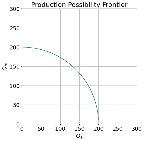
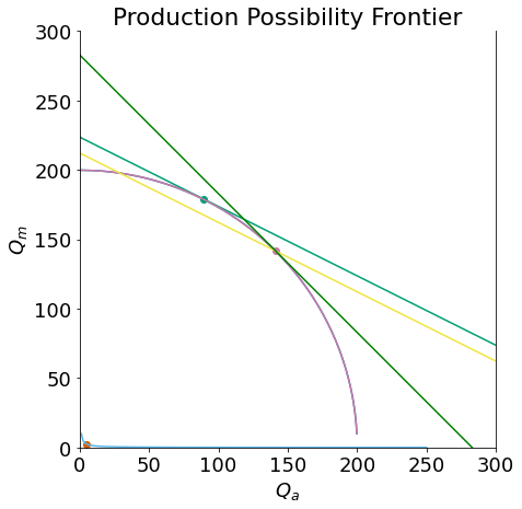
The production possibility frontier
We will use a bowed-out production possibility frontier. The details of how this is built don’t really matter to the analysis at hand but it will be easy to illustrate by leveraging our earlier analysis of the specific factors model.
Agriculture requires specific capital \(T\) and mobile labor:
Manufacturing production requires specific capital \(K\) and mobile labor:
The quantity of land in the agricultural sector and the quantity of capital in the manufacturing sector are both in fixed inelastic supply during the period of analysis.
The market for mobile labor is competitive and the market clears at a wage where the sum of labor demands from each sector equals total labor supply.
From this it is easy to build a production possibility frontier (to wit: at every level of \(L_A\) calculate and plot \(Q_a=F(K,L_a)\) and \(Q_m=G(K, \bar L - L_a)\).
See the SFM notebook for details on the parameters used to create these visualizations.
ppf(Tbar=100, Kbar=100, Lbar=400)
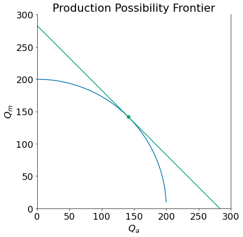
The closed economy
Let \(p\) be the relative price of manufactures
With the assumed technologies and parameters, the economy in autarky will have an autarky relative equilibrium price of \(p=1\) and would look like this:
open_trade(p=1, t = 0)
C:\Users\jconn\Anaconda3\lib\site-packages\scipy\optimize\minpack.py:175: RuntimeWarning: The iteration is not making good progress, as measured by the
  improvement from the last ten iterations.
  warnings.warn(msg, RuntimeWarning)
Production subsidy and tariff
An ad-valorem subsidy on manufactures of \(t\) will raises the effective price received by the domestic supplier from \(P_M\) to \(P_m(1+t)\). If we assume no tax or subsidy on agriculture then this also raises the relative price of manufactures from \(p\) to \(p(1+t)\).
A tariff can be thought of as a production subsidy to suppliers plus a consumption tax to consumers.
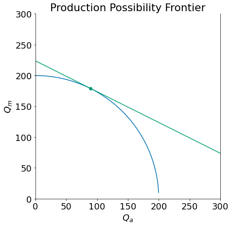
Suppose the small but closed economy with market equilibrium relative price \(p^a\) opens to trade. Since it is a small economy its own domestic prices will now be set by the world relative price, let’s call it \(p^w\).
The following diagram shows the open economy of a country which had a comparative advantage in the production of agricultural goods. As depicted as it opened to trade the relative price of manufactured goods falls from \(p=p^a=1\) to \(p=p^w=1/2\). We depict the market equilibrium (with no subsidy or tariff). As the price rises producers cut back on manufacturing production and expand agricultural production to take advantage of the price change. Meanwhile consumers substitute away from the now relatively more expensive agricultural good.
In this new equilibrium the country exports agricultural goods in exchange for manufactures.
open_trade(p=1/2, t = 0)
C:\Users\jconn\Anaconda3\lib\site-packages\scipy\optimize\minpack.py:175: RuntimeWarning: The iteration is not making good progress, as measured by the
  improvement from the last ten iterations.
  warnings.warn(msg, RuntimeWarning)
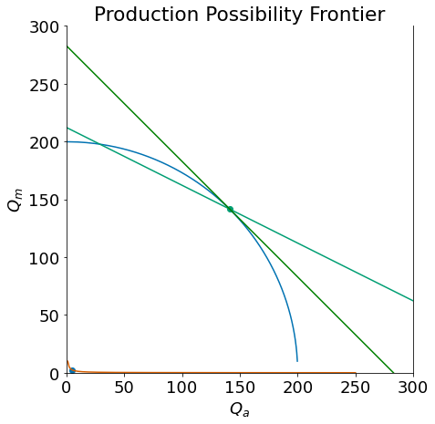
A production subsidy to manufacturers
The graph below depicts the effects of a production subsidy on equlibrium. Producers faced the distorted prices (steeper price line in graph below). The subsidy induced rise in the relative price of manufactures leads the economy to a new production point along the PPF (where the PPF is tangent to the new distorted price line). This production bundle is less valuable measured at world prices than the early bundle produced when the country followed it’s comparative advantage. That can be seen by comparing the world price line (national income at world prices) passing through this new bundle compared to a similar world price line passing through the free trade bundle that was chosen before the country distorted its domestic prices (not drawn below, but see the following figure) which can be seen to have higher intercepts (meaning measured in real terms in terms of either good national income is higher in the undistorted open economy equilibrium).
We can also see (see this and following diagram) how consumer welfare is reduced.
open_trade(p=1/2, t = 1, dt=True)
C:\Users\jconn\Anaconda3\lib\site-packages\scipy\optimize\minpack.py:175: RuntimeWarning: The iteration is not making good progress, as measured by the
  improvement from the last ten iterations.
  warnings.warn(msg, RuntimeWarning)
interact(open_trade, p=(0.25,2,0.25), t = (0,1,0.05) );
It gets a bit busy but if we draw the situation before and after on the same graph we can see clearly how the production subsidy, while it does raise the production of manufactures, also lowers national income measured at world prices as well as welfare.
open_trade(p=1/2, t = 0, dt=False)
open_trade(p=1/2, t = 1, dt=True)
C:\Users\jconn\Anaconda3\lib\site-packages\scipy\optimize\minpack.py:175: RuntimeWarning: The iteration is not making good progress, as measured by the
  improvement from the last ten iterations.
  warnings.warn(msg, RuntimeWarning)
C:\Users\jconn\Anaconda3\lib\site-packages\scipy\optimize\minpack.py:175: RuntimeWarning: The iteration is not making good progress, as measured by the
  improvement from the last ten iterations.
  warnings.warn(msg, RuntimeWarning)
def twoplot(t):
    open_trade(p=1/2, t = 0, dt=False)
    open_trade(p=1/2, t = t, dt=True)
interact(twoplot,t=(0,2,0.1));
A tariff
A tariff can be analyzed just as the production subsidy above, only that now consumers also face higher prices \(p(1+t)\).
The country still trades with the world at world prices \(p=p^w\) but consumers face the price distortion introduced by the tariff.
We don’t draw this situatino but look at the world price line (or national income line) at world prices running through the subsidy distorted production bundle. The country must trade along this line. But if consumers face distorted prices consumption must be at a point where the community indifference is tangent to these distorted price lines. Technically we can think of moving the distorted price line out parallel from the PPF along this world price line until we touch an indifference curve tangent to this distorted line. It’s easy to verify that this will take us to an indifference curve below the lowest indifference curve above. Hence we see that in addition to the deadweight loss (lost national income) from producing the wrong bundle of goods, when analysing a tariff, we also see the consumer loss of welfare from the consumer tax.