Increasing returns, Monopolistic Competition
Contents
Increasing returns, Monopolistic Competition
and International Trade
Here is a presentation and simulation of a model of “Increasing Returns to Scale, monopolistic competition and Trade” based on the Krugman (1979) article by the same name in the Journal of International Economics with the following simplifications and adaptations:
model and graph analysis simplified to be similar to Krugman, Obstfeld, Melitz textbook.
We use the linear demand setup from Salop, S. (1979) “Monopolistic Competition with Outside Goods,” Bell Journal of Economics
This is a jupyter notebook with executable python code for the graphs and simulations. If you want to execute and interact with the content below please first go to the Code Section below, execute the code there and then return. Also, if running on Microsoft azure notebooks ‘Change the kernel’ to python 3.6.
Preliminaries
Consider a demand curve of the form:
It’s associated inverse demand function will be: $\( P(q_i) = \frac{A}{b} - \frac{1}{b} \cdot q_i \)$
Total Revenue \(\mathit{TR}(q_i) = P(q_i) \cdot q_i\) can be differentiated to find $\( \mathit{MR}(q_i) = \frac{A}{b} - \frac{2}{b} \cdot q_i = P - \frac{1}{b} \cdot q_i \)$
and we can find an expression for the gap $\( P(q_i) - \mathit{MR}(q_i) = \frac{q_i}{b} \)$
This is also the firm’s markup over marginal cost \(P-\mathit{MC}\) (since \(\mathit{MR=MC}\)).
Note the larger is \(b\) the more firm sales fall for a given price rise (i.e. the more elastic is demand).
Firm Technology and Costs
Each firm has exclusive right to produce a unique product (protected by patent or copyright) but competitors can enter the market to supply similar goods. There is a relatively high fixed cost of establishing a production plant and then a simple constant marginal cost:
hence \(\mathit{MC}(q_i) = c\) and average cost is $\( AC(q_i) = \frac{F}{q_i} + c \)$
Demand for Product Variety
Consumers demand variety. Products are symmetric substitutes in consumption. Salop (1979) constructs a model with linear demands
assume symmetric demand for each good. Demand for firm \(i\)’s good is:
Here \(S\) is total output in the industry. If firm sets product price \(P_i\) equal to price of other similar products \(P\) then firm will produce \(q_i = \frac{S}{n}\) of total output. If it tries to raise \(P_i>P\) it loses some but not all market share.
Expanding out the earlier inverse demand equation:
which we can invert to get an inverse demand curve for each firm.
Monopolistically competitive market with entry will drive \(P=AC\) and hence profits to zero.
firm(S=S/20, F=F, c=c)
Solving for equilibrium \(n\) and \(\bar P\)
In a symmetric equilibrium \(P_i = \bar P\) then \(q_i = q = \frac{S}{n}\) or \(S = n \cdot q\)
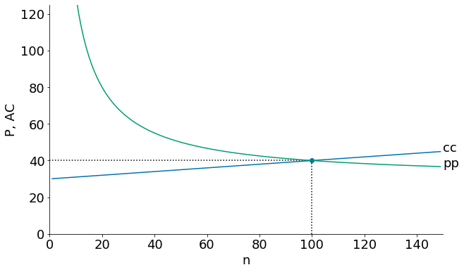
The cc curve
Average cost AC rises with the number of firms 𝑛 , because more firms in the same market means lower production runs and higher average fixed costs.
Substiting \(q = \frac{S}{n}\) into \(AC = \frac{F}{q} + c\)
Average cost rises with the number of firms \(n\) because each firm produces less \(\frac{S}{n}\) and so each firm is spreading their fixed costs over
The pp curve
Price falls with the number of firms 𝑛 because increased competition reduces markups.
In a symmetric equilibrium firm demand could be written $\( q_i = \left [\frac{S}{n} + b\bar P \right ] - S b P \\ q_i = A^\prime - b^\prime P \)$
Recall that with a demand curve of form \(q_i = A^\prime - b^\prime \cdot P\) we found a markup
Substituting using \(b^\prime = S\cdot b\), and \(q=\frac{S}{n}\) we get:
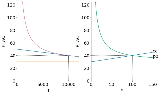
mkt_eq()
n = 100, P= 40, q = 10000, F/q = 10

interact(mkt_eq, S=(50*1000, 2000*1000,50*1000), F=fixed(F), c=fixed(c) );
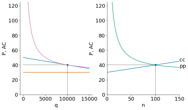
twopane(S,F,c);
n = 100, P= 40, q = 10000, F/q = 10
interact(twopane, S=(50*1000, 2000*1000,50*1000), F=fixed(F), c=fixed(c) );
Done
Code Section
import numpy as np
import matplotlib.pyplot as plt
from ipywidgets import interact, fixed
import seaborn as sns
plt.style.use('seaborn-colorblind')
plt.rcParams["figure.figsize"] = [6,6]
plt.rcParams["axes.spines.right"] = False
plt.rcParams["axes.spines.top"] = False
plt.rcParams["font.size"] = 18
plt.rcParams['figure.figsize'] = (10, 6)
plt.rcParams['axes.grid']=False
A = 100000
b = 1/1000
F = 100*1000
c = 30
S = 1*1000*1000
qmax = 100
nmax = 50
q = np.arange(1,qmax)
n = np.arange(1,nmax)
def p(q, A=A, b = b):
    return A/b - (1/b) * q
def mr(q, A=A, b = b):
    return A/b - (2/b) * q
def AC(q, F=F, c = c):
    return F/q + c
def mc(q, c = c):
    return c*np.ones(len(q))
def cc(n, S=S, F=F, c = c):
    return n*F/S + c
def pp(n, b=b,  c = c):
    return c + 1/(b*n)
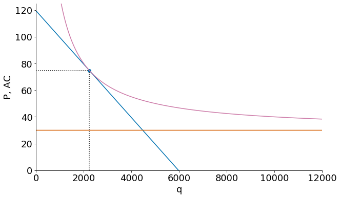
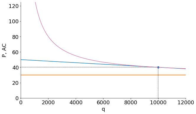
def firm(S =S, F=F, c=c):
    qmax = 15000
    ne = np.sqrt(S/(b*F))
    Pe = c + np.sqrt(F/(S*b))
    qe = S/ne
    q = np.arange(1,qmax)
    plt.xlim(0,12000)
    plt.ylim(0,125)
    plt.plot(q, p(q, A=(S/ne+b*S*Pe), b = b*S))
    plt.plot(q, mr(q, A, b))
    plt.plot(q, mc(q, c))
    plt.xlabel('q')
    plt.ylabel('P, AC')

    plt.plot(q, AC(q, F, c))
    plt.scatter(qe,AC(qe,F,c))
    plt.vlines(qe,0,Pe, linestyle=":")
    plt.hlines(Pe,0,qe, linestyle=":");
firm(S=S, F=F, c=c)
interact(firm, S=(50*1000, 2000*1000,50*1000), F=fixed(F), c=fixed(c));
def mkt_eq(S = S, F=F, c=c):
    nmax = 150
    n = np.arange(1,nmax)
    ne = np.sqrt(S/(b*F))
    Pe = c + np.sqrt(F/(S*b))
    AC = c + ne*F/S
    print(f"n = {ne:2.0f}, P={Pe:3.0f}, q = {S/ne:5.0f}, F/q = {ne*F/S:3.0f}")
    plt.xlim(0,150)
    plt.ylim(0,125)
    plt.xlabel('n')
    plt.ylabel('P, AC')
    plt.plot(n, cc(n, S=S, F=F, c = c))
    plt.plot(n, pp(n, b=b,  c = c))
    plt.text(nmax,pp(nmax),"pp")
    ntop = (100-c)*S/F
    plt.text(min(nmax,ntop), cc(min(ntop,nmax),S=S, F=F, c = c), "cc")
    plt.scatter(ne,Pe)
    plt.hlines(Pe,0,ne,linestyle=":")
    plt.vlines(ne,0,Pe,linestyle=":")
mkt_eq()
n = 100, P= 40, q = 10000, F/q = 10
interact(mkt_eq, S=(50*1000, 2000*1000,50*1000), F=fixed(F), c=fixed(c) )
<function __main__.mkt_eq(S=1000000, F=100000, c=30)>
def twopane(S, F, c):
    plt.figure()
    ax = plt.subplot(121)
    firm(S,F,c)
    ax= plt.subplot(122)
    mkt_eq(S,F,c);
twopane(S,F,c)
n = 100, P= 40, q = 10000, F/q = 10