A Model of Enclosures#
Matthew J. Baker and Jonathan Conning
Show code cell source
%load_ext autoreload
%autoreload 2

if 'google.colab' in str(get_ipython()):  # if using colab cloud must upload module file to their disk
  !wget https://raw.githubusercontent.com/jhconning/enclosure_book/main/notebooks/enclose.py
from enclose import *
plt.style.use('seaborn-ticks')
---------------------------------------------------------------------------
FileNotFoundError                         Traceback (most recent call last)
File /opt/hostedtoolcache/Python/3.11.13/x64/lib/python3.11/site-packages/matplotlib/style/core.py:129, in use(style)
    128 try:
--> 129     style = _rc_params_in_file(style)
    130 except OSError as err:

File /opt/hostedtoolcache/Python/3.11.13/x64/lib/python3.11/site-packages/matplotlib/__init__.py:903, in _rc_params_in_file(fname, transform, fail_on_error)
    902 rc_temp = {}
--> 903 with _open_file_or_url(fname) as fd:
    904     try:

File /opt/hostedtoolcache/Python/3.11.13/x64/lib/python3.11/contextlib.py:137, in _GeneratorContextManager.__enter__(self)
    136 try:
--> 137     return next(self.gen)
    138 except StopIteration:

File /opt/hostedtoolcache/Python/3.11.13/x64/lib/python3.11/site-packages/matplotlib/__init__.py:880, in _open_file_or_url(fname)
    879 fname = os.path.expanduser(fname)
--> 880 with open(fname, encoding='utf-8') as f:
    881     yield f

FileNotFoundError: [Errno 2] No such file or directory: 'seaborn-ticks'

The above exception was the direct cause of the following exception:

OSError                                   Traceback (most recent call last)
Cell In[2], line 2
      1 from enclose import *
----> 2 plt.style.use('seaborn-ticks')

File /opt/hostedtoolcache/Python/3.11.13/x64/lib/python3.11/site-packages/matplotlib/style/core.py:131, in use(style)
    129         style = _rc_params_in_file(style)
    130     except OSError as err:
--> 131         raise OSError(
    132             f"{style!r} is not a valid package style, path of style "
    133             f"file, URL of style file, or library style name (library "
    134             f"styles are listed in `style.available`)") from err
    135 filtered = {}
    136 for k in style:  # don't trigger RcParams.__getitem__('backend')

OSError: 'seaborn-ticks' is not a valid package style, path of style file, URL of style file, or library style name (library styles are listed in `style.available`)
Show code cell source
from ipywidgets import interact, interact_manual, fixed
Base Model#
Parameters#
\(\bar L\) : total labor supply
\(\bar T\) : total land supply
\(\bar l = \frac{\bar L}{\bar T}\) : population density
\(\theta\) : Expected TFP gain on enclosed land
\(\alpha\) : Labor intensity of production
Let \(T_e\) equal total land enclosed and \(t_e = \frac{T_e}{\bar T}\) the fraction of land enclosed.
Production Technologies#
On unenclosed land:
On enclosed land:
If \(\theta>1\) then enclosure would facilitate the adoption of higher productivity methods or technologies.
Enclosure cost At \(c\) cost per unit land ‘claimant’ can establish exclusive rights. The cost of enclosing \(T_e\) units of land is \(c\cdot T_e\).
Manufacturing sector: For now we start with an agriculture only economy with two subsectors: ‘enclosed’ and ‘unenclosed’. See the section below.
Open Access and/or Customary use-rights#
Both Weitzman (1974) and De Meza and Gould (1992) interpret unenclosed lands as open-access. But we can interpret this sector instead as a customary tenure regime with individualized use-rights. To see this note by Euler’s Theorem and linear homogeneity that we can write:
now divide by \(L\)
In other words the average product of labor earned in the unenclosed sector can be decomposed into earnings to labor plus implied land rents.
Think of the customary sector as a subeconomiy and assume there are competitive factor markets there:
From this and the earlier identity, we can write the value average product of labor earned by a worker in the customary sector as:
This can be explained with a ‘tenure insecurity’ interpretation. Workers establish and maintain rights of possession in the customary sector via continued possession and membership participation in the community. In the customary sector their labor earns the local wage \(w_c\) plus the implied rents from their share of unenclosed lands (assumed here to be equally divided, hence if there are \(T_c\) units of land and \(L_c\) workers in the sector, each gets \(T_c/L_c\) units of land to farm. We assume that the worker that leaves the customary sector to earn the enclosed sector can earn wage \(w_e\) there, but would lose any land and implied land rents held in the customary sector. We model the risk of losing land as certain now, but relax this assumption later.
Labor Market equilibrium#
As just described, the labor market is in equilibrium when workers are just indifferent between moving to earn in the enclosed and earning the wage \(w_e\) and remaining in the customary sector where they earn an average product:
This implies
The first inequality \(MPL_c<MPL_e\) implies a misallocation and ‘too much labor’ entering the unenclosed sector. This is a version of the so-called ‘tragedy’ of overuse).
The Enclosure decision#
Every piece of unenclosed land has a potential ‘owner-claimant.’
If they pay enclosure cost \(c\) they can exclude all other workers from the site.
They can then hire labor to maximize profits: \(\theta \cdot F_L(T_i, L_i) = w_e\)
‘Profits’ are the equivalent to rent on the now enclosed land.
It is profitable to enclose if \(r(t_e) > c\)
Since encloser faces wage \(w_e = p\cdot MPL_e > p\cdot MPL_c\)
hires fewer workers than were used under free access. Labor ‘shedding’
spillover: those released workers go ‘crowd’ remaining open access areas
Spillovers, strategic complementarities, multiple Nash equilibria:
Nobody encloses (and not profitable to deviate)
Everybody encloses (and not profitable to deviate)
The model#
Assume at first a purely agricultural economy
\(T_e, L_e\) – Amount of land enclosed, Ag. labor working on enclosed land.
\(t_e = \frac{T_e}{\bar T}\) – fraction of land enclosed
A useful decomposition#
\(F(t_e, l_e)\) tell us fraction of potential output for given land/labor enclosure \((t_e, l_e\))
Optimal Enclosures – The Planner’s problem#
Enclosure is costly so it is only worthwhile where the benefit from higher output/productivity compensates for the cost. The planner sets out to find the enclosure rate and land and labor allocations that maximize total benefits net of total costs:
FOC:
FOC:
At any level of \(t_e\) we can solve for the optimal labor across the enclosed and unenclosed sectors:
Note \(\Lambda^o=\theta^{\frac{1}{1-\alpha}}>1\) as \(\theta>1\)
If \(\theta = 1\) only way to equalize marginal products is via \(t_e=l_e\)
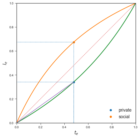
when \(\theta > 1\) then \(l_e^o(t_e)\) is concave down
Note that when \(\theta>1\), \(l_e \ge t_e\)
it is efficient to operate enclosed lands in more labor-intensive ways
Will soon show that (for \(1<\theta<\frac{1}{\alpha}\)) private enclosers have incentive to operate enclosed lands in less labor intensive ways than unenclosed lands!
Note we’ve added the option to have arbitrary renure security \(\mu\) parameter. Extent of security or exclusivity.
plotle(te = 0.48, th = 1.5, alp = 0.5, mu = 0)
0.34177215189873417 0.675
interact(plotle, te=(0,1,0.05), th=(0.5, 3, 0.1), alp =(0.2, 0.8, 0.05), mu=(0,1,0.1));
Planner Optimal enclosure rate \(t_e\)#
We can write
We will study output net of enclosure costs per unit land: \(z(t_e) - c \cdot t_e= \frac{Y(t_e)}{\bar T} - \frac{c \bar T t_e}{\bar T}\)
Note that \(\frac{F(\bar T, \bar L)}{\bar T} = \bar l^{\alpha}\) where \(\bar l=\frac{\bar L}{\bar T}\) represents population density.
We can simplify this to obtain:
We used some tricks to get to this simplified expression:
Derivation:
Step 1:
let’s break this into pieces like so:
Step 2, substitute in our expression for \(l_e(t_e)\) and note that first term A is:
and likewise
Note the last term on the right can be written:
And hence
We can simplify a lot by noticing that:
and
We can then write:
So we have:
Determining Optimal Enclosure#
If \(\Lambda^o=\theta^{\frac{1}{1-\alpha}} \ge 1\), (or simply \(\theta\ge 1\)), \(z(t_e)\) is concave down in \(t_e\).
That means we can determine the outcome just by looking at slope of \(z(t_e) -c \cdot te\)
That slope is given by:
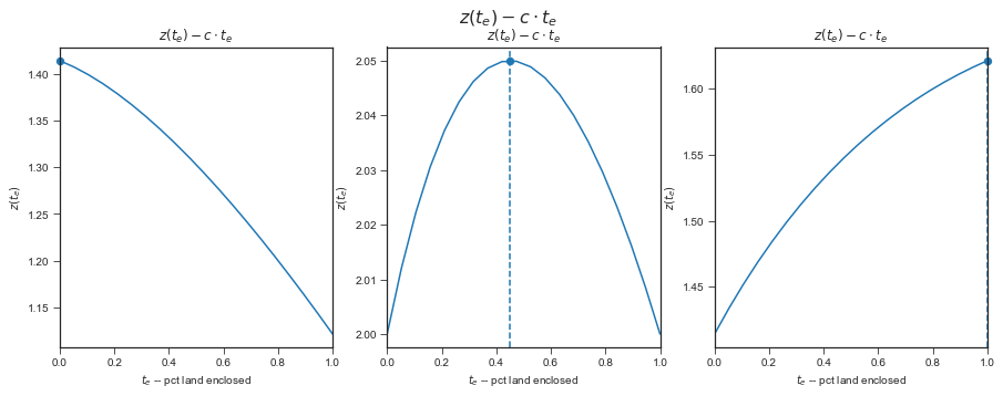
There are Three Cases#
Since z is concave The plots below draw \(z(t_e) - c \cdot t_e\)
Show code cell source
f, (ax1, ax2, ax3) = plt.subplots(1, 3, sharex=True, figsize=(15,5))
f.suptitle(r'$z(t_e)-c\cdot t_e$', fontsize=16)
ax1.set_title(r'Enclose None: $z(0)-c<0$')
ax1.set_ylabel(r'$z(t_e)$')
plotz(th = 1.5, alp=1/2, c=1, lbar=2,ax=ax1)
ax2.set_title(r'Partial: $z \prime (0)-c>0$ and $z \prime (1)-c<0$')
plotz(th = 1.5, alp=1/2, c=1, lbar=4, ax=ax2);
ax3.set_title(r'Enclose All: $z \prime (1)-c>0$')
plotz(th = 1.5, alp=1/2, c=0.5, lbar=2,ax=ax3);
Let’s examine these cases, one at a time:
(1) Enclose None (\(z'(0)-c<0\))#
plotz(th = 1.6, alp=1/2, c=1, lbar=1);
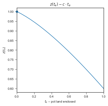
(1) Efficent No Enclosure: if \(z'(0)<c\) then \(z(t_e)-c\cdot t_e\) curve is everywhere downward sloping. In \(\theta\) by \(\bar l\) parameter space, this will be the case for all population densities \(\bar l\) that meet this inequality:
(2) Enclose all (\(z'(1)-c>0\))#
plotz(th = 1.8, alp=1/2, c=1, lbar=4);
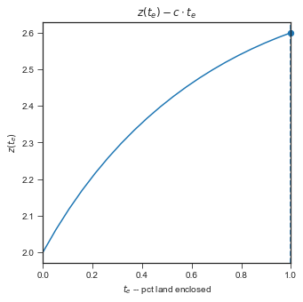
(2) Boundary of Full Enclosure Optimum: \(\bar l \ge \left[\frac{c \Lambda^o}{(1-\alpha)\left(\Lambda^o-1\right)}\right]^{\frac{1}{\alpha}}=l_1^o(c,\theta)\)
Partial enclosure \(z'(0)-c>0\) and \(z'(1)-c<0\)#
plotz(th = 1.7, alp=1/2, c=1, lbar=2);
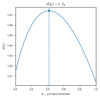
A widget to see how \(z(t_e)\) changes with parameter values:
interact(plotz, th=(0.5,2,0.1), alp=(0.2,0.8,0.1), c=(0,3,0.1), lbar = (1,3,0.1), ax=fixed(None));
Summarizing: optimal Enclosure decisions in \(\theta , \bar l\) parameter space#
\(\theta\) expected productivity gain
\(\bar l = \frac{\bar L}{\bar T}\) population density
(1) Boundary of No Enclosure Optimum: \(\bar l \le \left[\frac{c}{(1-\alpha)\left(\Lambda^o-1\right)}\right]^{\frac{1}{\alpha}}=l_0^o(c,\theta)\)
(2) Boundary of Full Enclosure Optimum: \(\bar l \ge \left[\frac{c \Lambda^o}{(1-\alpha)\left(\Lambda^o-1\right)}\right]^{\frac{1}{\alpha}}=l_1^o(c,\theta)\)
(3) Partial Enclosure Region: in between.
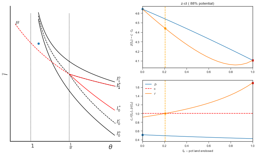
Here we see the two boundaries plotted. The dashed line boundaries correspond to the ‘conditional optimality’ boundaries, described in the paper.
allpart(soc_opt= True, cond_opt=True, pv_opt=False, pv_gg=False)
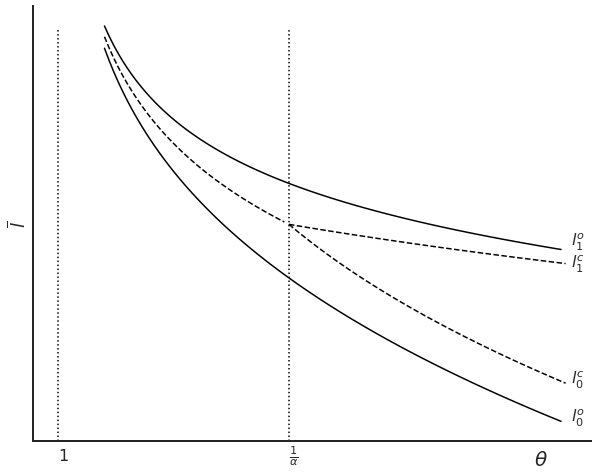
An interactive version of this plot is found further below.
Planner’s second-best benchmark#
States and local authorities might be able to regulate the rate of enclosure (t_{e}), but it may be much harder to regulate labor movement between the sectors. For example the government may designate an area such as a forest as protected but villagers or outsiders may still slip into the area to extract resources.
Accordingly, we ask: what is the second-best (or conditionally optimal) level of enclosure, when labor remains free
Solve for private economy \(l_e^*(t_e)\):
where
Note this is different from the first-best where \(\Lambda^o = \theta^\frac{1}{1-\alpha}\). \(l_e^*(t_e)\) is concave or convex depending on \(\Lambda \lessgtr 1\) or \(\theta\lessgtr \frac{1}{\alpha}\).
Once again we can find boundaries. Enclosure should begin if:
enclosure should be complete if:
These regions are plotted above.
Private decisions to enclose in a decentralized economy#
Owner-claimants independently and simultaneously decide whether to enclose each unit of land.
Displaced labor moves to remaining unenclosed lands (or manufacturing) until
Private claimant encloses if#
Low TFP gain case (i.e. \(\theta < \frac{1}{\alpha}\))#
\(r(t_e)\) is increasing in enclosure so long as \(\theta < \frac{1}{\alpha}\)
spillover across enclosers: as each ‘owner’ encloses pushes labor off land, lowering wage, raising return to enclosure by others.
Three parameter zones when \(\theta < \frac{1}{\alpha}\)
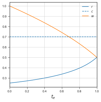
No private enclosure \(r(1)<c\)
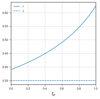
Full private enclosure \(r(0)>c\)
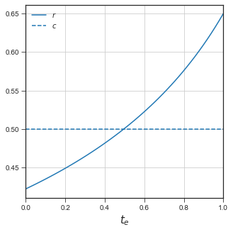
Multiple Equilibria (All enclose, None enclose) \(r(0)<c, r(1)>c\)
1. No private enclosure \(r(1)<c\)#
(low population density\(\bar l\), low expected productivity gain \(\theta\), and/or high enclosure costs \(c\))
plotreq(th = 1, alp=1/2, tlbar=1, c=0.7, wplot=True)
2.Full enclosure \(r(0)>c\)#
(high population density \(\bar l\) , high expected productivity gain \(\theta\) , and/or low enclosure costs \(c\))
plotreq(th = 1.25, alp=1/2, tlbar=1, c=0.35, wplot=False)
3. Multiple Equilibria#
Two Nash Equilibria:
Nobody encloses
Everybody encloses
plotreq(th = 1.3, alp=1/2, tlbar=1, c=0.5, wplot=False)
interact(plotreq,th=(0.8,2.5,0.05), alp=(0.2,0.8,0.1), tlbar=(0.5,5,0.1), c=(0,4,0.05), wplot=[True, False]);
Private Enclosure as a Global Game#
Enclosure Zones in the private Economy
allpart(c = 1, alp= 2/3, mu =0, soc_opt= True, cond_opt=False, pv_opt=True, pv_gg=True,logpop=True)

