Model Sketch#
Consider the following simple workhorse three-period consumption smoothing model where consumers’ preferences are summarized by constant relative risk aversion (CRRA) utility. In any period the consumer’s instantaneous utility is given by \(u(c)=c^{1-ρ}/(1-ρ)\). Over three period the agent maximizes utility
This is a version of the classic \(\beta-\delta\) quasi-hyperbolic discounting model. We assume the consumer has an autarky income stream \({y}=\{y_{0},y_{1},y_{2}\}\) which defines autarky or reservation utility \( \overline{u}(y) = U(y₀,y₁,y₂)\) but in general will prefer a smoother consumption profile from contracting on financial markets.
Contracts with and without commitment services#
Competitive full-commitment#
Let’s assume at first that financial intermediaries compete to offer a multiperiod contract and can – at zero cost – credibly commit to not renegotiate the terms of that contract. For the moment we also assume this contract to be enforceably exclusive in the sense that no other bank is allowed to offer a more attractive additional or alternative contract to the period 1 self. We’ll relax both assumptions shortly.
The offered contract will maximize the period-0 self’s present value of utility $\( U(c_{0},c_{1},c_{2})=u(c_{0})+\beta \left[ \delta u(c_{1})+\delta ^{2}u(c_{2})\right] \)$ subject to the bank’s zero profit condition or, same thing, consumer budget constraint:
At the optimal contract \(C^fc\) the consumer may save or borrow, depending on their initial income stream and preferred/feasible smoothed consumption stream available from contracting.
The first order conditions for an optimum are:
The optimal contract will be the three period consumption profile that brings the consumer to the highest feasible iso-utility surface (analogous to an indifference curve except in 3 dimensions), and that will be at a point where the iso-utility surface is tangent to the zero-profit hyperplane that cuts through endowment point \(y\)
For the CRRA case these can be rewritten as:
WLOG assume that \(\delta = \frac{1}{1+r}\) and \(r=0\) and hence \(\delta = 1\). This simplifies the expressions without changing the essential tradeoffs. $\( c_1 = c_2 = c_0 \beta ^\frac{1}{\rho} \)$
If we substitute the FOC \(c_1=c_2\) into the consumer’s binding budget constraint (the bank’s zero profit condition) the problem can be reduced from three equation (two FOC and the zero profit condition) to two:
The first equation highlight’s the period-zero self’s present bias –they want to consume more in period zer than in period one– while the second summarizes that hey want to smooth whatever resources are left to future consumption equally between periods 1 and 2.
Figure 1 below illustrates how the equilibrium contract is determined, drawn for the CRRA case where \(\beta=0.5\) and \(\rho = 1\) and \(\sum y =300\). The first of these two lines can be seen as the upward sloping income-expansion income-expansion line in the rightmost quadrant diagram in \(c_0\) and \(c_1\) space. The second line is seen as the downward sloping dashed line.
Note
To be continued
