Figure 3 Replication#
This page contains the code to replicate Figure 3 in the paper which shows captured ‘profits.’
A legal non-profit cannot distribute profits but, following the literature, we assume the commercial non-profit distributes ‘captured profits’ in the form of perquisites or other benefits to its directors.
Hybrid firms are for-profit firms with social-investors (e.g. mission-oriented non-profit shareholders in a for-profit microfinance firm)
Code#
Several functions used can be found in the python module Contract.py
import Contract
Code below uses this module to produce Figure 1. Code is hidden in HTML view. Click button to display.
import numpy as np
import matplotlib.pyplot as plt
from ipywidgets import interact, fixed
plt.rcParams['figure.figsize'] = 10, 8
np.set_printoptions(precision=2)
Commercial non-profits/hybrid ownership
Parameter \(\alpha\) summarizes the degree of ‘hybridity’ or non-profit orientation.
\(\alpha=1\): a pure for-profit firm where 100 percent of the raw profits can be captured and distributed by owner/shareholders.
\(\alpha=0\): pure non-profit. No profits can be captured and distributed for the benefit of owners.
\(0 < \alpha=0 < 1\): Hybrid ownership firm. A non-profit where fraction \(\alpha\) of raw profits are captured (e.g. indirectly via perquisites and other benefits) or a hybrid ownership firm (e.g. B-corporation or a for-profit that has significant non-profit shareholders, as is quite common in modern microfinance).
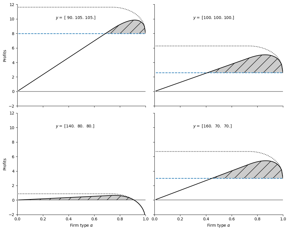
A ‘pure’ for profit (with \(\alpha\)=1.0) earns a reduced (possibly negative) profit due to it’s inability to commit. Seen in the plot as profits the height of the horizontal line.
Any non-profit with \(\alpha\) above about 0.4 and below 1.0 can better commit to not renegotiate a larger set of contracts and therefore can offer a more profitable renegotiation-proof contract. Even though they capture only fraction \(\alpha\) of those profits, the take home profits exceed the profits of the pure for-profit.
THe no-renegotiation constraint is:
We will illustrate with a ‘non-pecuniary’ sanction (e.g. guilt or mission-drift penalty)
Where \(B\) is a constant, for example \(B = \bar \kappa\)
This implies that the managers/board of a pure for-profit firm feel no non-pecuniary sanction at renegotiating a contract but a firm of type \(\alpha <1\) does incur a sanction for breaching commitments they’d made in period 0. This then implies that we can now write the no-renegotiation constraint as:
where \(\kappa(\alpha) = \frac{\eta(\alpha)}{\alpha}\)
Given our earlier stated choice of \(\eta(\alpha) = 10 \cdot (1 - \alpha)\) we will therefore use in the illustrated contracts below:
This is monotonically decreasing in \(\alpha\) from prohibitively high as \(\alpha \rightarrow 0\) as \(\kappa(\alpha) \rightarrow 0\) to \(\kappa(1) = 0\).
Figure 3 plot#
def hybrid_plot(y0=100, beta=0.65, rho=1.01, ax = None):
    cM     = Contract.Monopoly(beta=beta)
    cM.rho = rho

    cM.y      = np.array([y0, (300-y0)/2, (300-y0)/2])
    num       = 100
    alphs     = np.linspace(0.01, 1, num)      # step through different values of alpha

    eta =  10*(np.ones(num) - alphs)   # eta(alpha) = 10*(1-alpha)  non-pecuniary
    KA  =  eta/alphs                   # kappa(alpha)

    cMRP      = np.zeros((3,num))          # initialize matrices to store iterated values for later plot
    zeros     = np.zeros(num)
    pvRP      = np.zeros(num)
    pvaRP     = np.zeros(num)
    pvRP_full = np.zeros(num)


    for i in range(num):
        cM.kappa = KA[i]                    # change optimal contract
        cMRP[:,i] = cM.reneg_proof()
        pvRP[i] = cM.PV(cM.y - cMRP[:,i])   # raw profit
        pvaRP[i] = alphs[i] * pvRP[i]       # captured profit  = alpha * raw

    pvRP_full = pvRP[-1]*np.ones(num)       # pure profit level (alpha=1)

    if ax is None:
        ax = plt.gca()

    ax.plot(alphs, pvRP_full,'--', label='pure for-profit')
    ax.plot(alphs, pvRP, label='raw profit', linestyle=':', color='black')
    ax.plot(alphs, pvaRP, label='captured profit', color='black')
    ax.plot(alphs, zeros, label='zero profit', color='black', alpha=0.5)
    ax.text(0.3,10, f'$y = $ {cM.y}')

    if ax is None:
        ax = plt.gca()
        ax.set_title(r'Captured Profits by firm type $\alpha$')
        ax.set_xlabel(r'firm type $ \alpha$', fontsize=11)
        ax.set_ylabel('Captured Profit', fontsize=11)
        ax.legend(loc='upper center', bbox_to_anchor=(0.5, -0.1),
          fancybox=None, ncol=5)
    ax.spines['right'].set_visible(False)
    ax.spines['top'].set_visible(False)

    if pvRP[-1]>0:
        ax.fill_between(alphs, np.fmax(pvaRP, pvRP_full), pvRP_full, hatch='/', facecolor='grey', alpha=0.4)
    else:
        ax.fill_between(alphs, np.fmax(pvaRP, zeros), zeros, hatch='/', facecolor='grey', alpha=0.4)

    ax.set_xlim(0,1)
    ax.set_ylim(-2,12)
# make figure with subplots
f, ax = plt.subplots(2, 2, sharex=True, figsize=(10,8))
beta = 0.65
rho = 1.05
hybrid_plot(y0=90, beta=beta, rho=rho, ax = ax[0,0])
hybrid_plot(y0=140, beta=beta, rho=rho, ax = ax[1,0])
hybrid_plot(y0=100, beta=beta, rho=rho, ax = ax[0,1])
hybrid_plot(y0=160, beta=beta, rho=rho, ax = ax[1,1])

ax[1,0].set_xlabel(r"Firm type $\alpha$")
ax[0,0].set_ylabel(r"Profits")
ax[1,0].set_ylabel(r"Profits")
ax[0,1].set_yticklabels([])
ax[1,1].set_xlabel(r"Firm type $\alpha$")
ax[1,1].set_yticklabels([])
f.savefig('Figure3.pdf')
f.tight_layout();
Interactive Plot and gif#
In order for the widget sliders to affect the chart you must be running this on a jupyter notebooks server. If you are viewing this on the web, click on the Rocket icon button above to launch a cloud server service (Binder, or google colab).
interact(hybrid_plot, y0=(50, 200, 5), beta=(0.4, 0.95, 0.05), rho=(0.501, 1.501, 0.1), ax=fixed(None));
A gif to illustrate how the plot adjusts to parameter changes: