Hechscher-Ohlin-Samuelson

Hechscher-Ohlin-Samuelson#

Model of Trade#

See the Edgeworth Box notebook to understand how the Edgeworth Box diagrams drawn below were constructed to represent this economy.

from hos import *

Small Open Economy#

Consider a small-open economy with two production sectors – agriculture and manufacturing – with production in each sector taking place with constant returns to scale production functions. Producers in the agricultural sector maximize profits

max_{K_{A}, L_{A}} p_{A} F (K_{A}, L_{A}) - w L_{A} - r K_{A}

Producers in manufacturing maximize

max_{K_{M}, L_{M}} p_{M} F (K_{M}, L_{M}) - w L_{M} - r K_{M}

In equilibrium total factor demands must equal total supplies:

K_{A} + K_{M} = \bar{K}

L_{A} + L_{M} = \bar{L}

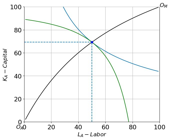
Here is an [Edgeworth Box](Edgeworth.ipynb_ that depicts the situation where $L_{A} = 50$ units of labor are allocated to the agricultural sector and all other allocations are efficient (along the efficiency locus).

edgeplot(50)

(LA,KA)=(50.0, 69.2)  (QA, QM)=(60.8, 41.2)  RTS= 2.1

../../_images/424ebbcf5a692cdc308055c9226fc77c402f644229bbb79fa5b002ed9e7b3afa.png

If you’re reading this using a jupyter server you can interact with the following plot, changing the technology parameters and position of the isoquant. If you are not this may appear blank or static.

LA = 50
interact(edgeplot, LA=(10, Lbar-10,1), 
         Kbar=fixed(Kbar), Lbar=fixed(Lbar),
         alpha=(0.1,0.9,0.1),beta=(0.1,0.9,0.1));

Resource Allocation in a small open economy#

From the first order conditions for profit maximization in each sector we have:

P_{A} F_{L} (K_{A}, L_{A}) = w = P_{M} G_{L} (K_{M}, L_{M})

Note this condition states that competition has driven firms to price at marginal cost in each industry or $P_{A} = M C_{A} = w \frac{1}{F_{L}}$ and $P_{M} = M C_{M} = w \frac{1}{G_{L}}$ which in turn implies that at a market equilibrium optimum

\frac{P_{A}}{P_{M}} = \frac{G_{L} (K_{M}, L_{M})}{F_{L} (K_{A}, L_{A})}

This states that the world price line with slope (negative) $\frac{P_{A}}{P_{M}}$ will be tangent to the production possibility frontier which as a slope (negative) $\frac{M C_{A}}{M C_{M}} = \frac{P_{A}}{P_{M}}$ which can also be written as $\frac{G_{L}}{F_{L}}$ or equivalently $\frac{G_{K}}{F_{K}}$ . The competitive market leads producers to move resources across sectors to maximize the value of GDP at world prices.

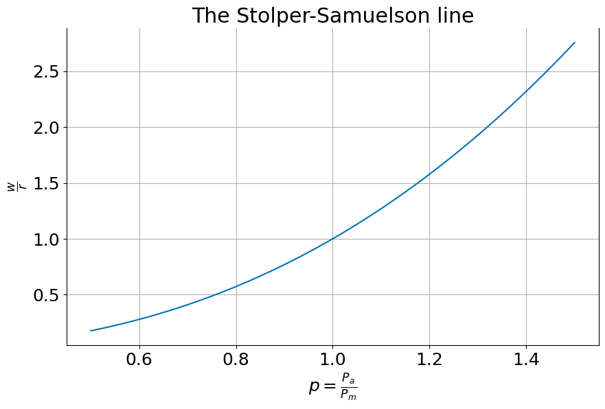
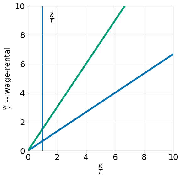
The Stolper Samuelson line#

We can derive a relationship between relative product prices (set on the world market) and the equilibrium wage-rental ration $w / r$ .

With the Cobb Douglas technology we can write:

F_{L} = (1 - α) {[\frac{K_{A}}{L_{A}}]}^{α}

F_{K} = α {[\frac{L_{M}}{K_{M}}]}^{α}

The first order necessary conditions for an interior optimum in each sector lead to an equilibrium where the following condition must hold:

\frac{F_{L} (K_{A}, L_{A})}{F_{K} (K_{A}, L_{A})} = \frac{w}{r} = \frac{G_{L} (\bar{K} - K_{A}, \bar{L} - L_{A})}{G_{K} (\bar{K} - K_{A}, \bar{L} - L_{A})}

Using these expressions and earlier factor demand expressions we can derive:

\frac{P_{A}}{P_{M}} = \frac{1 - α}{1 - β} \frac{{[\frac{(1 - β)}{β} \frac{w}{r}]}^{β}}{{[\frac{(1 - α)}{α} \frac{w}{r}]}^{α}}

or

\frac{P_{A}}{P_{M}} = Γ {[\frac{w}{r}]}^{β - α}

where

Γ = \frac{1 - α}{1 - β} {(\frac{α}{1 - α})}^{α} {(\frac{1 - β}{β})}^{β}

Inverting, we get an expression for the Stolper Samuelson Line

\frac{w}{r} = \frac{1}{Γ} {[\frac{P_{A}}{P_{M}}]}^{\frac{1}{β - α}}

The Stolper Samuelson Theorem#

The Stolper Samuelson theorem tells us how changes in the world relative price of products translates into changes in the relative price of factors and therefore in the distribution of income in society.

The theorem states that an increase in the relative price of a good will lead to an increase in both the relative and the real price of the factor used intensively in the production of that good (and conversely to a decline in both the real and the relative price of the other factor).

This relationship can be seen from the formula. If agriculture were more labor intensive than manufacturing, so $α < β$ , then an increase in the relative price of agricultural goods creates an incipient excess demand for labor and an excess supply of capital (as firms try to expand production in the now more profitable labor-intensive agricultural sector and cut back production in the now relatively less profitable and capital-intensive manufacturing sector). Equilibrium will only be restored if the equilibrium wage-rental ratio falls which in turn leads firms in both sectors to adopt more capital-intensive techniques. With more capital per worker in each sector output per worker and hence real wages per worker $\frac{w}{P_{a}}$ and $\frac{w}{P_{m}}$ increase.

ssline(a=0.3, b=0.7)

../../_images/56724d3d7c33694bd495e48e9781d547688b091cdd3db2790a418e4bd4b837f4.png

Solving for equilibrium allocation as a function of relative price p#

Code to solve for unique HOS equilibrium as a function of world relative price $\frac{P_{A}}{P_{M}}$

From Lerner-Edgeworth box

Equilibrium in the capital market: $ $K_{a} + K_{m} = \bar{K}$ $

We can use $K_{a} = k_{a} \cdot L_{a}$ and $K_{m} = k_{m} \cdot L_{a}$ to rewrite this as:

k_{a} \cdot L_{A} + k_{m} \cdot L_{m} = \bar{K}

Noting that $L_{m} = \bar{L} - L_{a}$ and solving for $L_{a}$

k_{a} \cdot L_{A} = \bar{K} - k_{m} \cdot (\bar{L} - L_{A})

L_{A} = \frac{\bar{K} - k_{m} \cdot \bar{L}}{k_{a} - k_{m}}

We now have enough to solve the model. If the economy is open to trade, it takes factor prices as given. For example if the $\frac{P_{a}}{P_{m} = 1}$ then we fan find $w / r$ and from that optimal capital intensities in each industry $k_{a}$ and $k_{m}$

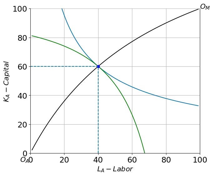
When $\frac{P_a}{P_m}=1, \frac{w}{r}$ = 1.00 and $(k_a, k_m)$ = (0.43, 2.33)

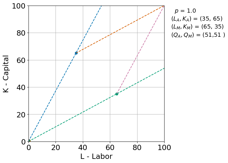
HOS(1)

(LA,KA)=(40.0, 60.0)  (QA, QM)=(51.0, 51.0)  RTS= 2.2

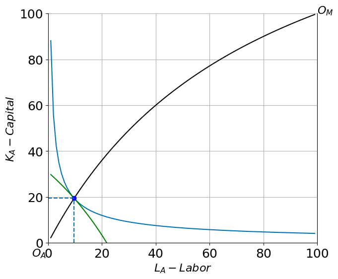
../../_images/fb899fab635c4d3c5660a754f252417917bda4508c75d1b337f55df84d20b29d.png

HOS(1.06)

(LA,KA)=( 9.7, 19.4)  (QA, QM)=(14.7, 86.3)  RTS= 3.0

../../_images/40228dc595a847980a6e900ea4e3a799f93b9d7e06ff928772112ee857d32444.png

interact(HOS, p=(0.8, 1.1,0.01), 
         Kbar=fixed(Kbar), Lbar=(90, 150,10),
         alpha=(0.1,0.5,0.1), beta=(0.5,0.9,0.1));

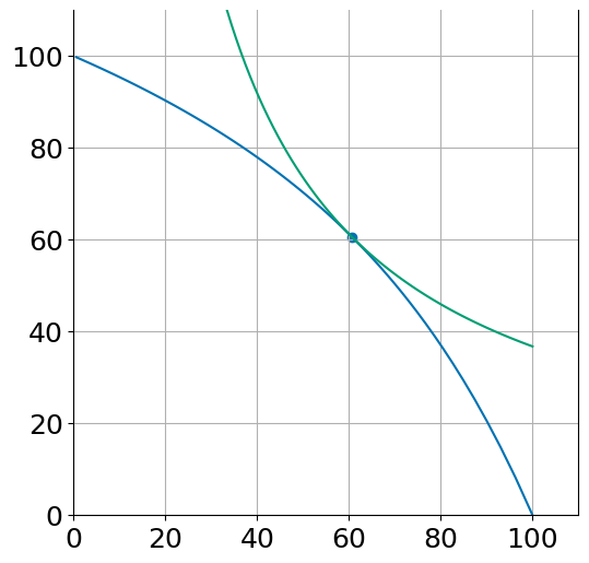
klplot(1)

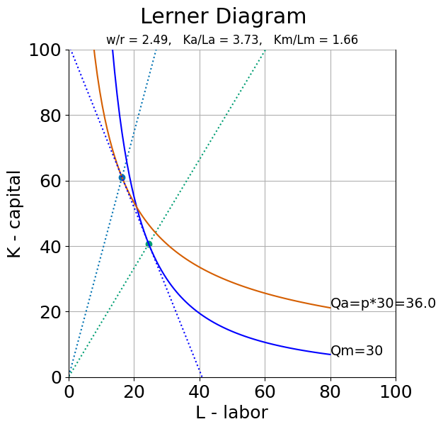
../../_images/93d5c6144bc8f9f8eb63784a406e39ff331e0bd995682309e11101507aabc30b.png

lerner(p=1.2)

w/r = 2.49, KLa = 3.73, KLm = 1.66

../../_images/8b04d0b3bc107d4c0e892882816a07e97865a00d864bb4e1f391381dcb6fe507.png

interact(lerner, p=(0.7,1.4,0.1));

closed_plot(alpha=0.8, beta=0.2)

(Qa, Qm) = (60.6, 60.6)

../../_images/02a11bf88256c3ddfdea7091dd2a84ae4e4f20a34815e57eeacb54bab3eccde5.png

interact(closed_plot, alpha=(0.1,0.9,0.1), beta=(0.1,0.9,0.1));

NOTE: Something is off on this Rybyczynski Edgeworth plot… had been working..

rybplot(1, Kbar=Kbar, Lbar=Lbar, alpha=0.65, beta=0.35)

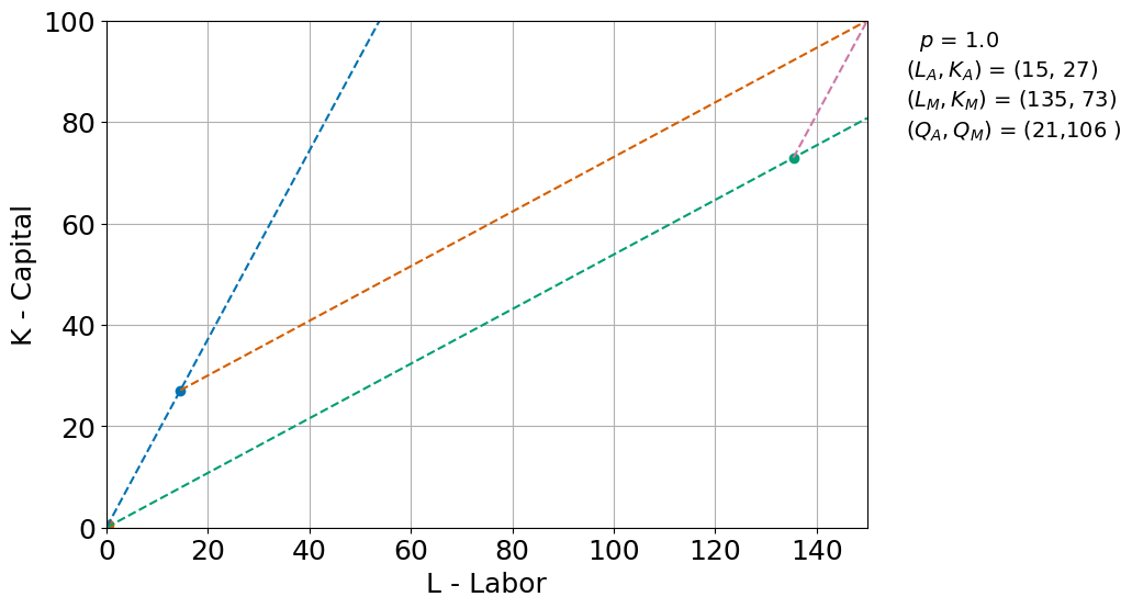
../../_images/82d303bab69fc2b67d838e202282e2ba4e0287e38d854be4a6f4be6ed5f87607.png

Rbyczynski Theorem. Adding labor should more than proportionately expand the productinon of the labor-intensive product and reduce the production of the other good. Here Manufacturing is the labor-intensive sector. We added increase $\bar{L}$ from 100 to 150 and we see how in the new equilibrium labor in manufacturing goes up from $L_{M} = 65$ to $L_{M} = 135$ . Output of manufacturing increases from 51 to 106 and output of agriculture falls from 51 to 21.

rybplot(1, Kbar=Kbar, Lbar=Lbar*1.5, alpha=0.65, beta=0.35)

../../_images/f5132d2f58135bb2aa1d47c5fcd0503d7edf958878614fc4cd6dea384e522e46.png

interact(rybplot, p = fixed(1), Lbar =(50,150,10), Kbar =(50,150,10), alpha=fixed(0.65), beta=fixed(0.35));