Edgeworth Box - Teaching Economics

Production allocation efficiency¶

from hos import *

Model Parameters¶

The model uses these parameters (defined in hos.py):

$\alpha$ = 0.6: Capital share in agriculture (sector A)
$\beta$ = 0.4: Capital share in manufacturing (sector M)
$\bar{K}$ = 100: Total capital endowment
$\bar{L}$ = 100: Total labor endowment

Since $\alpha > \beta$ , agriculture is relatively capital-intensive compared to manufacturing.

from hos import *

Efficiency in production¶

Consider a small-open economy with two production sectors -- agriculture and manufacturing -- with production in each sector taking place with constant returns to scale production functions. Producers in the agricultural sector maximize profits

\max_{K_A,L_A} p_A F(K_A,L_A) - w L_A - r K_A

(1)

Producers in manufacturing maximize

\max_{K_M,L_M} p_M G(K_M,L_M) - w L_M - r K_M

(2)

In equilibrium total factor demands must equal total supplies:

K_A + K_M = \bar K

(3)

L_A + L_M = \bar L

(4)

The first order necessary conditions for an interior optimum in each sector lead to an equilibrium where the following condition must hold:

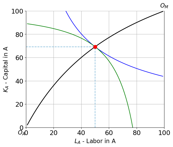
\frac{F_L(K_A,L_A)}{F_K(K_A,L_A)} = \frac{w}{r} =\frac{G_L(\bar K-K_A,\bar L- L_A)}{G_K(\bar K-K_A,\bar L- L_A)}

(5)

Efficiency requires that the marginal rates of technical substitution (MRTS) be equalized across sectors (and across firms within a sector which is being assumed here). In an Edgeworth box, isoquants from each sector will be tangent to a common wage-rental ratio line.

If we assume Cobb-Douglas forms $F(K,L) = K^\alpha L^{1-\alpha}$ and $G(K,L) = K^\beta L^{1-\beta}$ the efficiency condition can be used to find a closed form solution for $K_A$ in terms of $L_A$ :

\frac{(1-\alpha)}{\alpha}\frac{K_A}{L_A} =\frac{w}{r} =\frac{(1-\beta)}{\beta}\frac{\bar K-K_A}{\bar L-L_A}

(6)

Here is an Edgeworth Box depicting the situation where $L_A = 50$ units of labor are allocated to the agricultural sector and all other allocations are efficient (along the efficiency locus).

Edgeworth Box plots¶

edgeplot(50)

(LA, KA) = (50.0, 69.2)  (QA, QM) = (60.8, 41.2)  RTS =  2.1

The Production Possibility Frontier¶

The efficiency locus also allows us to trace out the production possibility frontier: by varying $L_A$ from 0 to $\bar L$ and, for every $L_A$ , calculating $K_A(L_A)$ and with that efficient production $(Q_A,Q_M)$ where $Q_A=F(K_A(L_A), L_A)$ and $Q_M=G(\bar K - K_A(L_A), \bar L - L_A)$ .

The curvature of the PPF depends on how different the factor intensities are:

When $\alpha \approx \beta$ (similar factor intensities): PPF is nearly straight
When $\alpha \gg \beta$ or $\alpha \ll \beta$ (very different intensities): PPF is more curved

For Cobb-Douglas technologies the PPF will be quite straight unless $\beta$ and $\alpha$ are very different from each other. In practical terms, this means that quite small changes to product prices will move production around quite a bit when factor intensities are similar.

ppf(30, alpha=0.9, beta=0.1)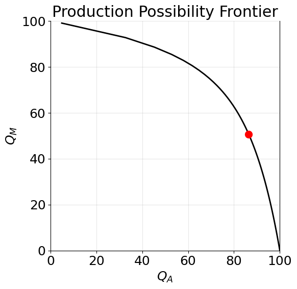

Jump to the notebook on the Heckscher-Ohlin-Samuelson to see a very practical application of the Edgeworth Box and this basic model framework and derive a number of theorems regarding how a small open economy will respond to a change in world relative prices or factor endowments.

If you’re reading this using a jupyter server you can interact with the following plot, changing the technology parameters and position of the isoquant. If you are not this may appear blank or static.

LA = 50
interact(edgeplot, LA=(10, Lbar-10,1), 
         Kbar=fixed(Kbar), Lbar=fixed(Lbar),
         alpha=(0.1,0.9,0.1),beta=(0.1,0.9,0.1));

Loading...

The Production Possiblity Frontier¶

The efficiency locus also allows us to trace out the production possibility frontier: by varying $L_A$ from 0 to $\bar L$ and, for every $L_A$ , calculating $K_A(L_A)$ and with that efficient production $(q_A,q_B)$ where $q_A=F(K_A(L_A), L_A)$ and $q_B=F(\bar K - K_A(L_A), \bar L - L_A)$ .

For Cobb-Douglas technologies the PPF will be quite straight unless $\beta$ and $\alpha$ are very different from each other! (In practical terms what this means is that quite small changes to product prices will move around production quite a bit)

ppf(30,alpha =0.9, beta=0.1)

Jump to the notebook on the Hecksher-Ohlin-Samuelson to see a very practical application of the Edgeworth Box and this basic model framework and derive a number of theorems regarding how a small open econonomy will respond to a change in world relative prices or factor endowments.