The CES Production Function - Teaching Economics

This notebook provides an introduction to the Constant Elasticity of Substitution (CES) production function, showing how it generalizes many familiar production functions including Cobb-Douglas, Leontief, and linear production functions.

This notebook was created with assistance from Claude.

Learning Objectives¶

After working through this notebook, you will be able to:

Understand the mathematical form of the CES production function
Explain the relationship between the substitution parameter ρ and the elasticity of substitution σ
Recognize how the CES function nests other production functions as special cases
Visualize and interpret isoquants for different elasticities of substitution
Understand how factor substitutability affects production choices

import numpy as np
import matplotlib.pyplot as plt
from ipywidgets import interact, FloatSlider, IntSlider
from scipy.optimize import fsolve

%matplotlib inline
plt.rcParams['figure.figsize'] = (10, 6)

The CES Production Function¶

The CES production function is given by:

Y = A\left[\alpha K^{\rho} + (1-\alpha) L^{\rho}\right]^{\frac{1}{\rho}}

(1)

where:

$Y$ is output
$K$ is capital input
$L$ is labor input
$A > 0$ is a productivity parameter (total factor productivity)
$\alpha \in (0,1)$ is a distribution parameter (share parameter)
$\rho \leq 1$ is the substitution parameter

The Elasticity of Substitution¶

The key feature that gives the CES function its name is that the elasticity of substitution between capital and labor is constant and related to ρ by:

\sigma = \frac{1}{1-\rho}

(2)

or equivalently:

\rho = \frac{\sigma - 1}{\sigma}

(3)

The elasticity of substitution $\sigma$ measures how easy it is to substitute between capital and labor while keeping output constant. Higher values of σ mean the inputs are more substitutable.

Alternative Representation Using σ¶

Because the elasticity of substitution σ has a more direct economic interpretation than ρ, the CES production function is sometimes written directly in terms of σ. Substituting $\rho = \frac{\sigma-1}{\sigma}$ into the production function yields:

Y = A\left[\alpha K^{\frac{\sigma-1}{\sigma}} + (1-\alpha) L^{\frac{\sigma-1}{\sigma}}\right]^{\frac{\sigma}{\sigma-1}}

(4)

Both representations are equivalent - they describe the same production technology. The ρ-form is more compact, while the σ-form makes the economic interpretation clearer:

When $\sigma = 0$ : The exponents become $-\infty$ , giving Leontief (perfect complements)
When $\sigma = 1$ : The exponents become 0/1, giving Cobb-Douglas
When $\sigma \to \infty$ : The exponents approach 1, giving perfect substitutes

In this notebook, we’ll primarily use the ρ-form for implementation, but you’ll see both forms in the economics literature. Trade economists and growth theorists often prefer the σ-form, while those doing numerical work often use the ρ-form.

Special Cases¶

The CES function is remarkably general and includes several familiar production functions as special cases:

Case	$\rho$	$\sigma$	Production Function	Name
Perfect Complements	$\rho \to -\infty$	$\sigma = 0$	$Y = A\min(K, L)$	Leontief
Cobb-Douglas	$\rho \to 0$	$\sigma = 1$	$Y = A K^{\alpha} L^{1-\alpha}$	Cobb-Douglas
Perfect Substitutes	$\rho = 1$	$\sigma \to \infty$	$Y = A[\alpha K + (1-\alpha)L]$	Linear

Intuition:

When σ = 0 (Leontief): Capital and labor must be used in fixed proportions (like one driver per truck)
When σ = 1 (Cobb-Douglas): Moderate substitutability (the most commonly used case)
When σ → ∞ (Linear): Capital and labor are perfect substitutes (like two types of identical workers)

Implementing the CES Production Function¶

Let’s implement the CES production function and its special cases:

def ces_production(K, L, A=1, alpha=0.5, rho=0.5):
    """
    CES production function.
    
    Parameters:
    -----------
    K : array-like
        Capital input
    L : array-like
        Labor input
    A : float
        Total factor productivity (default=1)
    alpha : float
        Distribution parameter, must be in (0,1) (default=0.5)
    rho : float
        Substitution parameter, must be ≤ 1 (default=0.5)
    
    Returns:
    --------
    Y : array-like
        Output
    """
    return A * (alpha * K**rho + (1-alpha) * L**rho)**(1/rho)

def cobb_douglas(K, L, A=1, alpha=0.5):
    """
    Cobb-Douglas production function (special case of CES when rho=0).
    """
    return A * K**alpha * L**(1-alpha)

def leontief(K, L, A=1):
    """
    Leontief production function (perfect complements, sigma=0).
    """
    return A * np.minimum(K, L)

def linear(K, L, A=1, alpha=0.5):
    """
    Linear production function (perfect substitutes, sigma=infinity).
    """
    return A * (alpha * K + (1-alpha) * L)

def rho_from_sigma(sigma):
    """
    Convert elasticity of substitution to substitution parameter.
    """
    return (sigma - 1) / sigma

def sigma_from_rho(rho):
    """
    Convert substitution parameter to elasticity of substitution.
    """
    return 1 / (1 - rho)

Visualizing CES Isoquants¶

An isoquant shows all combinations of capital and labor that produce the same level of output. The shape of the isoquant reveals how substitutable the inputs are:

More curved (bowed toward origin): Lower σ, harder to substitute
Less curved (closer to straight line): Higher σ, easier to substitute
L-shaped: σ = 0 (Leontief, perfect complements)
Straight line: σ → ∞ (perfect substitutes)

Let’s create a function to compute and plot isoquants:

def compute_isoquant(Y_target, L_range, A=1, alpha=0.5, rho=0.5):
    """
    Compute capital needed for each labor level to achieve target output.
    
    For CES: Y = A[alpha*K^rho + (1-alpha)*L^rho]^(1/rho)
    Solving for K:
    K = [(Y/A)^rho - (1-alpha)*L^rho) / alpha]^(1/rho)
    """
    L_range = np.array(L_range)
    
    # Handle special cases
    if rho == 1:  # Perfect substitutes
        K = (Y_target/A - (1-alpha)*L_range) / alpha
        return L_range, K
    
    # General CES case
    # K = [(Y/A)^rho - (1-alpha)*L^rho) / alpha]^(1/rho)
    term = (Y_target/A)**rho - (1-alpha) * L_range**rho
    
    # Only keep positive values
    valid = term > 0
    L_valid = L_range[valid]
    K_valid = (term[valid] / alpha)**(1/rho)
    
    return L_valid, K_valid

def plot_isoquants(sigma_values, Y_target=10, A=1, alpha=0.5, L_max=30):
    """
    Plot isoquants for different elasticities of substitution.
    """
    fig, ax = plt.subplots(figsize=(10, 6))
    
    L_range = np.linspace(0.1, L_max, 500)
    
    for sigma in sigma_values:
        # Handle special cases first to avoid division by zero
        if sigma == 0:  # Leontief
            # L-shaped isoquant
            L_vals = np.array([0, Y_target/A, Y_target/A, L_max])
            K_vals = np.array([Y_target/A, Y_target/A, 0, 0])
            label = f'σ = {sigma:.1f} (Leontief)'
        elif sigma == 1:  # Cobb-Douglas (approximate with rho close to 0)
            rho = 0.001  # Use small rho to approximate Cobb-Douglas
            L_vals, K_vals = compute_isoquant(Y_target, L_range, A, alpha, rho)
            label = f'σ = {sigma:.1f} (Cobb-Douglas)'
        elif np.isinf(sigma):  # Perfect substitutes
            rho = 1
            L_vals, K_vals = compute_isoquant(Y_target, L_range, A, alpha, rho)
            label = f'σ = ∞ (Perfect Substitutes)'
        else:
            # General CES case - now safe to call rho_from_sigma
            rho = rho_from_sigma(sigma)
            L_vals, K_vals = compute_isoquant(Y_target, L_range, A, alpha, rho)
            label = f'σ = {sigma:.2f}'
        
        ax.plot(L_vals, K_vals, linewidth=2, label=label)
    
    ax.set_xlabel('Labor (L)', fontsize=12)
    ax.set_ylabel('Capital (K)', fontsize=12)
    ax.set_title(f'CES Isoquants for Different Elasticities of Substitution\n(Output = {Y_target}, α = {alpha})', fontsize=14)
    ax.legend(loc='upper right', fontsize=10)
    ax.grid(True, alpha=0.3)
    ax.set_xlim(0, L_max)
    ax.set_ylim(0, L_max)
    
    plt.tight_layout()
    plt.show()

Comparing Key Special Cases¶

Let’s first compare the three main special cases side by side:

# Compare Leontief, Cobb-Douglas, and Perfect Substitutes
plot_isoquants(sigma_values=[0, 1, np.inf], Y_target=10, alpha=0.5)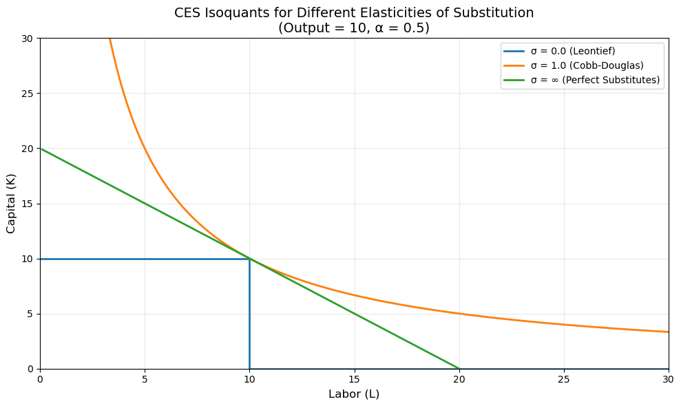

Interpretation:

σ = 0 (Leontief, red line): L-shaped isoquant. Capital and labor must be used in fixed proportions. No substitution is possible - if you have 10 units of labor, you need exactly 10 units of capital to produce the target output, regardless of relative prices.
σ = 1 (Cobb-Douglas, orange curve): Moderate curvature. This is the “benchmark” case. You can substitute capital for labor (or vice versa), but with diminishing returns. This is the most commonly used production function in economics.
σ = ∞ (Perfect Substitutes, green line): Straight line. Capital and labor are perfect substitutes. You can freely exchange one for the other at a constant rate. For example, two types of workers who are equally productive.

The Full Spectrum of Substitutability¶

Now let’s see how isoquants change as we vary σ across a wider range:

# Show a spectrum of sigma values
plot_isoquants(sigma_values=[0.3, 0.5, 1, 2, 4, 10], Y_target=10, alpha=0.5)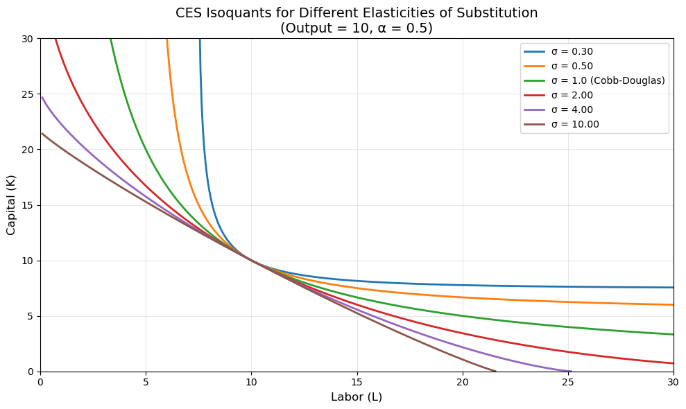

Interpretation:

As σ increases (moving from red to purple in the plot):

Low σ (0.3, 0.5): Isoquants are very curved. Inputs are complements - you need both capital and labor, and it’s hard to substitute one for the other. Examples: drivers and trucks, computers and electricity.
σ = 1: The Cobb-Douglas benchmark. Moderate substitutability.
High σ (2, 4, 10): Isoquants become increasingly straight. Inputs are good substitutes. Examples: different types of fuel, different varieties of similar crops, skilled workers who can perform similar tasks.

The curvature of the isoquant tells us about production flexibility: flatter isoquants mean more flexibility to adjust the capital-labor ratio in response to changing input prices.

Interactive Exploration¶

Use the interactive widget below to explore how the elasticity of substitution affects the shape of the isoquant:

@interact(
    sigma=FloatSlider(min=0.1, max=5.0, step=0.1, value=1.0, description='σ'),
    alpha=FloatSlider(min=0.1, max=0.9, step=0.1, value=0.5, description='α'),
    Y_target=IntSlider(min=5, max=20, step=1, value=10, description='Output'),
)
def interactive_isoquant(sigma=1.0, alpha=0.5, Y_target=10):
    """
    Interactive plot of a single CES isoquant.
    """
    fig, ax = plt.subplots(figsize=(10, 6))
    
    L_range = np.linspace(0.1, 30, 500)
    rho = rho_from_sigma(sigma)
    
    # Compute isoquant
    L_vals, K_vals = compute_isoquant(Y_target, L_range, A=1, alpha=alpha, rho=rho)
    
    # Plot
    ax.plot(L_vals, K_vals, linewidth=3, color='darkblue', label=f'Y = {Y_target}')
    
    # Add reference point
    L_ref = Y_target
    if rho != 1:
        K_ref = ((Y_target)**rho - (1-alpha) * L_ref**rho) / alpha
        if K_ref > 0:
            K_ref = K_ref**(1/rho)
            ax.plot(L_ref, K_ref, 'ro', markersize=10, label=f'L={L_ref:.1f}, K={K_ref:.1f}')
    
    ax.set_xlabel('Labor (L)', fontsize=12)
    ax.set_ylabel('Capital (K)', fontsize=12)
    ax.set_title(f'CES Isoquant: σ = {sigma:.2f}, α = {alpha:.2f}, ρ = {rho:.3f}', fontsize=14)
    ax.legend(loc='upper right', fontsize=11)
    ax.grid(True, alpha=0.3)
    ax.set_xlim(0, 30)
    ax.set_ylim(0, 30)
    
    # Add interpretation text
    if sigma < 0.5:
        substitutability = "Very low substitutability (strong complements)"
    elif sigma < 1:
        substitutability = "Low substitutability (complements)"
    elif sigma == 1:
        substitutability = "Moderate substitutability (Cobb-Douglas)"
    elif sigma < 2:
        substitutability = "Moderate-high substitutability"
    else:
        substitutability = "High substitutability (good substitutes)"
    
    ax.text(0.02, 0.98, substitutability, transform=ax.transAxes,
            fontsize=11, verticalalignment='top',
            bbox=dict(boxstyle='round', facecolor='wheat', alpha=0.5))
    
    plt.tight_layout()
    plt.show()

The Marginal Rate of Technical Substitution (MRTS)¶

The slope of the isoquant at any point is called the Marginal Rate of Technical Substitution (MRTS). It tells us how much capital we can give up for one additional unit of labor while keeping output constant:

MRTS_{L,K} = -\frac{dK}{dL}\bigg|_{Y=\bar{Y}} = \frac{MP_L}{MP_K}

(5)

For the CES production function:

MRTS_{L,K} = \frac{1-\alpha}{\alpha} \left(\frac{K}{L}\right)^{1-\rho}

(6)

Key insight: The MRTS depends on the capital-labor ratio (K/L) and the substitution parameter ρ:

When ρ is close to 1 (high σ): MRTS is nearly constant → isoquant is nearly straight
When ρ is very negative (low σ): MRTS changes dramatically with K/L → isoquant is very curved
When ρ = 0 (Cobb-Douglas): MRTS = (1-α)/α → moderate curvature

def mrts(K, L, alpha=0.5, rho=0.5):
    """
    Marginal Rate of Technical Substitution for CES production function.
    MRTS = (1-alpha)/alpha * (K/L)^(1-rho)
    """
    return ((1-alpha)/alpha) * (K/L)**(1-rho)

@interact(
    sigma=FloatSlider(min=0.2, max=3.0, step=0.2, value=1.0, description='σ')
)
def plot_mrts(sigma=1.0):
    """
    Plot MRTS as a function of the capital-labor ratio.
    """
    fig, ax = plt.subplots(figsize=(10, 6))
    
    K_L_ratio = np.linspace(0.1, 5, 100)
    rho = rho_from_sigma(sigma)
    alpha = 0.5
    
    # Compute MRTS for each K/L ratio
    mrts_vals = ((1-alpha)/alpha) * K_L_ratio**(1-rho)
    
    ax.plot(K_L_ratio, mrts_vals, linewidth=3, color='darkgreen')
    ax.set_xlabel('Capital-Labor Ratio (K/L)', fontsize=12)
    ax.set_ylabel('MRTS', fontsize=12)
    ax.set_title(f'Marginal Rate of Technical Substitution\nσ = {sigma:.2f}, ρ = {rho:.3f}', fontsize=14)
    ax.grid(True, alpha=0.3)
    ax.set_ylim(0, 5)
    
    # Add interpretation
    if sigma == 1:
        text = "Cobb-Douglas: MRTS proportional to K/L"
    elif sigma > 1:
        text = f"High σ: MRTS less sensitive to K/L (flatter)"
    else:
        text = f"Low σ: MRTS very sensitive to K/L (steeper)"
    
    ax.text(0.5, 0.95, text, transform=ax.transAxes,
            fontsize=11, verticalalignment='top',
            bbox=dict(boxstyle='round', facecolor='lightblue', alpha=0.5))
    
    plt.tight_layout()
    plt.show()

Summary and Economic Applications¶

Key Takeaways¶

The CES production function generalizes many familiar cases: It includes Leontief (σ=0), Cobb-Douglas (σ=1), and linear production (σ→∞) as special cases.
The elasticity of substitution σ governs factor substitutability:
- Low σ: Factors are complements (must be used together)
- High σ: Factors are substitutes (easily interchangeable)
Isoquant shapes reveal production flexibility:
- Curved isoquants (low σ): Firms have less flexibility to adjust input ratios
- Straight isoquants (high σ): Firms can easily adjust input ratios

Economic Applications¶

The CES production function is used extensively in:

Growth theory: Understanding how economies respond to changes in capital and labor supplies
International trade: Modeling how countries with different factor endowments specialize
Labor economics: Analyzing substitution between skilled and unskilled labor
Environmental economics: Studying substitution between clean and dirty inputs
Development economics: Examining technology adoption and factor substitution in agriculture

Why Does σ Matter?¶

The elasticity of substitution has important implications:

Factor prices: When σ is low, changes in factor supplies have large effects on relative prices
Income distribution: The value of σ affects how economic growth is shared between capital and labor
Technological change: Whether technical progress is capital-augmenting or labor-augmenting matters more when σ ≠ 1
Policy responses: A firm’s ability to respond to taxes or regulations depends on how easily it can substitute inputs

Further Exploration¶

Try experimenting with the interactive widgets above to develop intuition for:

How the α parameter shifts the isoquant’s position
How different industries might have different σ values
What happens to cost minimization when input prices change for different values of σ