The \bar \kappa Threshold

$\bar \kappa$ is the threshold minimum renegotiation cost that is required to sustain a first best efficient smoothing contract. Any $\kappa < \bar \kappa$ will require some endogenous distortion of the contract to keep the contract renegotiation-proof.

If a contract $(c_1^0,c_2^0)$ is renegotiated it would be to a new contract $(c_1, c_2)$ that maximizes one-self’s preferences. Hence, a renegotiation-proof contract would satisfy the constraint:

u(c_{1}^{0})+\beta u(c_{2}^{0}) \ge u(c_1) + \beta u(c_2)

(1)

Let’s substitute on the right hand side for the best $c_1, c_2$ contract that one-self can obtain. One-self wants

u'(c_1) = \beta u'(c_2)

(2)

For the CRRA case, this implies $c_2 = \beta^{\frac{1}{\rho}} \cdot c_1$ . The most favorable renegotiated contract for one-self would leave the renegotiating bank indifferent (after subtracting out the renegotiation cost):

c_1 + c_2 = c_1^0 + c_2^0 - \kappa

(3)

Since we just pointed out that $c_2 = \beta^{\frac{1}{\rho}} \cdot c_1$ , this can be rewitten as:

c_1 = \frac{c_1^0 + c_2^0 - \kappa}{1 + \beta^\frac{1}{\rho}}

(4)

Notice also that $\beta u(c_2) = \beta u(\beta^{\frac{1}{\rho}} \cdot c_1)$ can be written $\beta u(c_2)=\beta^{\frac{1}{\rho}}u(c_1)$ Putting this all together, the no-renegotiation constraint above can be rewritten as:

u(c_{1}^{0})+\beta u(c_{2}^{0})\le u\left(\frac{c_{1}^{0}+c_{2}^{0}-\kappa}{1+\beta^{\frac{1}{\rho}}}\right)(1+\beta^{\frac{1}{\rho}})

(5)

A first-best efficient contract $will be: C_0^F=(c_0^F, c_1^F, c_2^F)$ with $c_1^F=c_2^F$ .

Let’s substitute that into the no-renegotiation constraint above. With appropriate simplifications such as $c_1^F=c_2^F$ we can write:

u(c_1^F)(1+\beta) \le u\left(\frac{2 \cdot c_1^F-\kappa}{1+\beta^{\frac{1}{\rho}}}\right)(1+\beta^{\frac{1}{\rho}})

(6)

For this CRRA case, we can solve further:

c_1^F \cdot \left ( 1+\beta^\frac{1}{\rho} \right)^\frac{1}{1-\rho} \le \frac{2 \cdot c_1^F-\kappa}{1+\beta^{\frac{1}{\rho}}} \cdot \left ( 1+\beta \right)^\frac{1}{1-\rho}

(7)

Re-arranging to solve for the $\kappa=\bar \kappa$ at which this holds as an equality, we find:

Setting $c_{1}^{0} =c_1^F = c_{2}^{0}$ equal to the implied efficient continuation contract into no-renegotiation constraint we can solve for the $\bar \kappa$ value of $\kappa$ that allows this to just hold:

\bar \kappa = c_1^F \cdot \Upsilon

(8)

where

\Upsilon=\left[2-\left[\frac{(1+\beta)}{\left(1+\beta^{\frac{1}{\rho}}\right)^{\rho}}\right]^{\frac{1}{1-\rho}}\right]

(9)

The above is for the competitive case.

For the monopoly case we simply replace the competitive $c_1^F$ term by the analogous $c_1^{mF}$ efficient monopoly contract ters. The monopoly formula for the threshold is thus $\bar \kappa^m = c_1^{mF} \cdot \Upsilon$

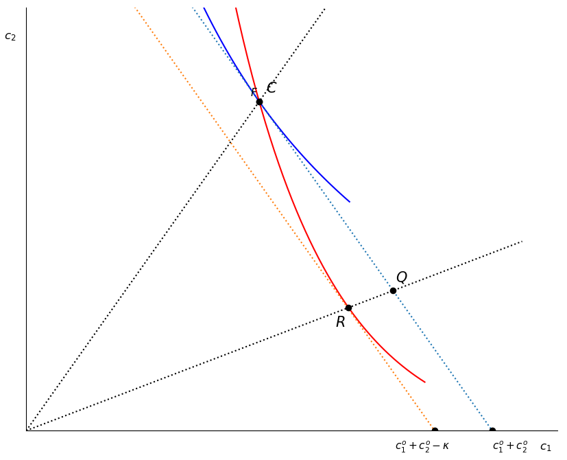
This diagram helps to visualize. Zero’s first-best commitment smoothing contract at $F$ is not because the $\kappa =\bar \kappa$ renegotiation cost is just high enough to make the bank reject the most favorable renegotiated contract that could be offered to the bank at $R$ .

Code¶

Several functions used can be found in the python module Contract.py

import Contract

Code below uses this module to produce Figure 1. If code is hidden in HTML view, click button to display.

import numpy as np
import matplotlib.pyplot as plt
from ipywidgets import interact,fixed
plt.rcParams['figure.figsize'] = 10, 8
np.set_printoptions(precision=2)

Competitive $\bar \kappa$ and Monopoly $\bar \kappa^M$ ¶

We will in general have $\bar \kappa^M \le \bar \kappa$

Cc = Contract.Competitive(beta=0.6)
Cm = Contract.Monopoly(beta=0.6)

Cc.kbar(), Cm.kbar()

(4.43642366042653, 4.3219284107549765)

def plotkb(rho=0.9, y0 = 100):
    num = 40
    kb = np.zeros(shape=(num, 3))
    Cc.y = np.array([y0, (300-y0)/2, (300-y0)/2])
    Cm.y = np.array([y0, (300-y0)/2, (300-y0)/2])
    Cc.rho = rho
    Cm.rho = rho
    for i in range(num):
        Cc.beta = i/num
        Cm.beta = i/num
        kb[i] = np.array([i/num, Cc.kbar(), Cm.kbar()])
    
    plt.plot(kb[:,0], kb[:,1], label = 'competitive')
    plt.plot(kb[:,0], kb[:,2], label = 'monopoly')
    plt.legend()
    plt.xlabel(r'$\beta$', fontsize=14)
    plt.ylabel(r'$\bar \kappa, \bar \kappa^m$', fontsize=14)
    plt.xlim(0,1)
    plt.ylim(0,20)

plotkb(rho = 1.1, y0 = 100)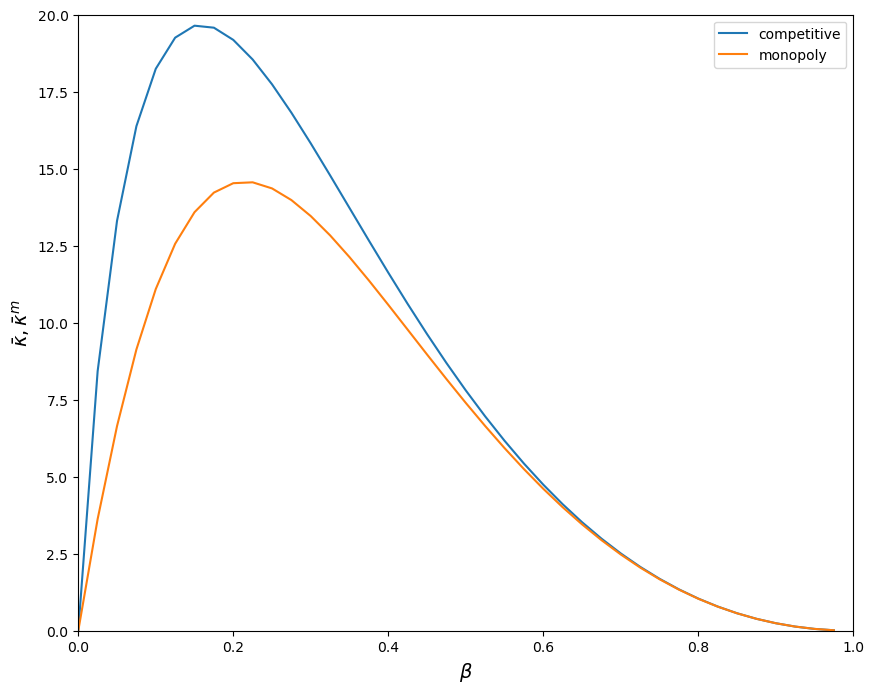

Interactive Plot¶

In order for the widget sliders to affect the chart you must be running this on a jupyter notebooks server. If you are viewing this on the web, click on the Rocket icon button above to launch a cloud server service (Binder, or google colab).

interact(plotkb, rho=(0.1, 2, 0.101), y0=(50,300,10));

Loading...

Code¶

Competitive κˉ\bar \kappaκˉ and Monopoly κˉM\bar \kappa^MκˉM¶

Interactive Plot¶

Competitive $\bar \kappa$ and Monopoly $\bar \kappa^M$ ¶