The Ricardian Trade Model

This is one in a series of python jupyter notebooks on Trade models by Jonathan Conning

Notes: the plots and simulations below are written in python. This notebook can be run interactively on a jupyter server, on your own machine or on a cloud serve such as Google’s Colab. However, much of the code is in a separate ricardo.py module. You can also view this notebook in slideshow mode (Alt-R) if the proper extension is installed.

Warm up: Budget lines and Indifference curves¶

You have I=$100 income. You can buy good X or good Y (for example good X might be food nutrition bars and good Y manufactured trinkets).

• $p_x$ -- Price of one unit of good X measured in $ per unit

• $p_y$ -- Price of one unit of good Y measured in $ per unit

• $\frac{p_x}{p_y}$ -- Relative price of good X measured in units of good Y per unit of X.

Interactive: Move the sliders to change prices and income values.

Ricardian model¶

Linear Production Technologies¶

Labor is the only input. Good $X$ and good $Y$ are produced with linear production technologies:

where $MPL_X$ and $MPL_X$ are the constant marginal product of labor productivity parameters in the $X$ and the $Y$ sector, respectively.

The marginal product of good $X$ is measured in units of good $X$ per unit labor.

The labor resource constraint¶

The sum of labor demands in the two sectors cannot exceed the economy’s total labor supply $\bar L$:

Minimum labor requirements¶

We can invert the $X$ production function to find the minimum labor required to produce any quantity $Q_X$:

$a_{LX}=\frac{1}{MPL_X}$ is the constant unit labor requirement to produce each additional unit of $Q_X$.

The minimum labor required to produce any quantity $Q_Y$ is

$a_{LY}=\frac{1}{MPL_Y}$ is the constant unit labor requirement to produce each additional unit of $Q_Y$.

The Production Possibility Frontier (PPF)¶

Tells us what is feasible to produce given available technology and resource constraints.

The economy’s labor resource constraint

can be rewritten (using our minimum labor requirement functions) to find:

Let’s re-arrange the PPF constraint further to obtain an expression that will be easy to plot:

Example: If $MPL_X = 2$, $MPL_Y = 1$ and $\bar L = 200$ then the PPF curve is given by:

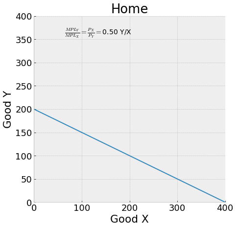
The PPF has:

• $Y$ intercept: $MPL_Y \cdot \bar L = 1 \cdot 200 = 200$

• $X$ intercept: $MPL_X \cdot \bar L = 2 \cdot 200 = 400$

The negative slope shows that there is a tradeoff:

• We need $\frac{1}{MPL_X}=1/2$ workers to produce one more unit of good X.

• With full employment we can only get this labor by pulling them out of Y production.

• Each worker there would have produced $MPL_Y=1$ units of Y, so withdrawing $\frac{1}{MPL_X}$ workers will reduce Y output by

Hence (negative of) the slope tells us the opportunity cost of an extra unit of good X, measured in terms of units of good Y which must be given up.

Competitive Prices and Wages¶

Firms will earn profit and want to hire more workers so long as the marginal value product of labor exceeds the market wage. Competition between firms and workers moving across firms and sectors in search of the highest wage will drive profits to zero at which the following market equilibrium conditions must hold:

All workers are paid the same wage which will be equal to their marginal value product, which is equalized across firms and sectors.

Real wages¶

The nominal wage $w$ is measured in dollars. From the zero profit condition we can determine real wages:

These are two ways to measure the purchasing power of this nominal wage in terms of good $X$ and good $Y$ respectively.

In this competitive economy workers are paid a real wage equal to their marginal product (which in the Ricardian model is also equal to their average product). Workers are the only factor of production and firm profits are driven to zero so workers get all of the output in the economy.

Note: $\frac{w}{P_X}$ and $\frac{w}{P_Y}$ are not different wages for workers in each sector. They are just two different ways to measure the real purchasing power of a worker’s wage $w$. There is only one wage in the economy and all workers earn the same wage no matter what sector or firm they work in!

It’s easy to determine real wages from just eyeballing the PPF graph, if you know the size of the labor force. In the plot real GDP measured in terms of good X is 400 units and since there are 100 workers each worker gets paid a real wage of 4 units of X. If real GDP is measured instead in terms of good Y real GDP is 200 units of Y and since there are 100 workers each worker gets paid a real wage of 2 units of Y.

We could also define a real wage in terms of any arbitrary basket of goods. For example, let

be the price of a basket with one unit of good $X$ and one of good $Y$. The wage $w$ can purchase $\frac{w}{P_B}$ such baskets.

Prices in the closed economy¶

To produce one unit of $X$ requires $a_{LX}=\frac{1}{MPL_X}$ units of labor. Each unit of labor costs $w$. Hence the marginal cost of producing $X$ is

Cmpetitive firms maximize profits where $P_X=MC_x$ and hence:

Similarly in sector $Y$, firms price at:

So the domestic (or closed economy) relative price of $X$ measured in terms of good $Y$ is

which is equal to the slope of the PPF. Relative prices reflect opportunity costs.

Note that in this Ricardian model with linear production technologies we have determined equilibrium relative prices without having to specify consumer preferences or demand! This will not be the case in more general models.

Interactive diagram¶

Visible/interactive if running a jupyter server.

Home opens to Trade -- Gains to Trade¶

Suppose Home has these technologies and resources:

Then the opportunity cost of producing one unit of good X measured in terms of good Y at Home is:

This is Home’s autarky relative price of producing good X

If the world relative price of good X is $\frac{p_x^w}{p_y^w} = 1$ units of Y then Home is a relatively low cost producer of good X (since 1/2 units of Y per X < 1 units of Y per X). Given Home’s technologies and these world prices Home has a comparative advantage in the production of good X

If it opens up to trade producers will find it profitable to continue to expand X production (at the expense of Y production) until the country becomes specialied in the production of X. At that point the country’s GDP will be $MPL_X \cdot \bar L$ units of good X which it can trade to the world at the world price of 1 unit of good Y per X. Hence the citizens of the Home country can consume along the consumption possibility frontier given by the world price line running through the specialization point $(q_x=MPL_x\cdot \bar L and q_y = 0)$

The specialized economy is depicted below.

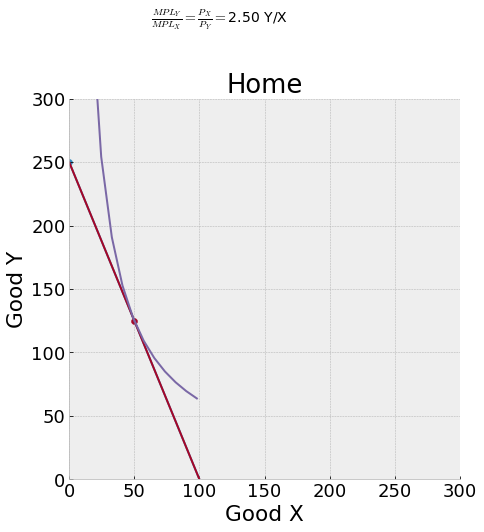
A two country model¶

Technologies and hence domestic relative prices are different in two countries.

At Home:

In Foreign:

The autarky relative price of X is

At HOME: $\frac{MPL_Y}{MPL_X} = \frac{1}{2}$ units of good Y per X

In FOREIGN: $\frac{MPL_Y^*}{MPL_X^*} = \frac{2}{1}$ units of good Y per X

Home has a comparative advantage at producing X as it is the lower cost producer.

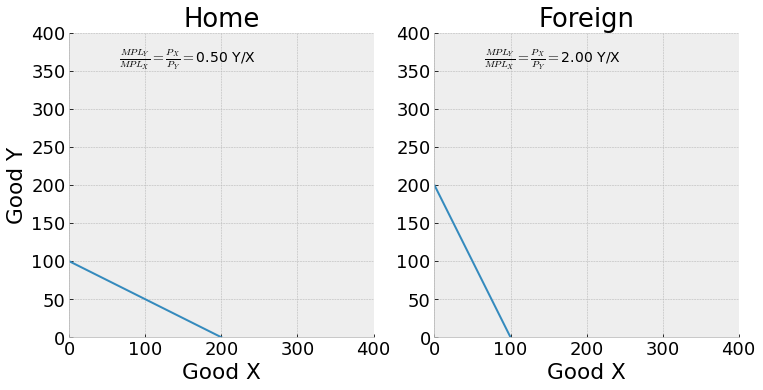
At a world price of $\frac{p_x^*}{p_y^*}=\frac{3}{4}$ units of good Y per X, Home will specialize at X production and Foreign at Y production, but trade will not balance.

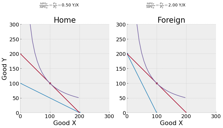
World Equilibrium Prices¶

Broadly speaking, the world equilibrium price will be that price at which one country’s exports equal the other country’s imports. It should be pretty clear that it will lie somewhere between the closed-economy relative prices of each country. In the example above Home autarky relative price of good X was $\frac{P_x}{P_y}=\frac{1}{2}$, the foreign autarky relative price was $\frac{P_x}{P_y}=2$ and the world equilibrium price that balances trade is $\frac{P_x^e}{P_y^e}=1$.

Since we can determine the quantity of exports and imports in each country at any world price, we could try to find the equilibrium price by trial and error -- by increasing or decreasing the world relative price until trade balances. Let’s start with that idea:

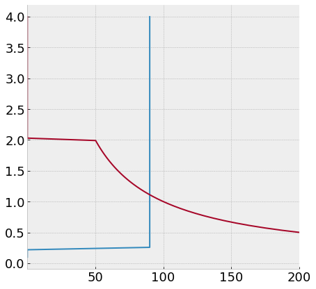
To find a world equilibrium price consistent with balanced trade we only need to find where the market for one good clears. The worldeq function finds this relative price numerically as the price at which world excess demand for good X is to zero.

The worldeq finds the world equilibrium price.